Analyze NYC yellow taxi data with DuckDB on Parquet files from S3

This example shows how to use Modal for a classic data science task: loading table-structured data into cloud stores, analyzing it, and plotting the results.

In particular, we’ll load public NYC taxi ride data into S3 as Parquet files, then run SQL queries on it with DuckDB.

We’ll mount the S3 bucket in a Modal app with CloudBucketMount. We will write to and then read from that bucket, in each case using Modal’s parallel execution features to handle many files at once.

Basic setup

You will need to have an S3 bucket and AWS credentials to run this example. Refer to the documentation for the exact IAM permissions your credentials will need.

After you are done creating a bucket and configuring IAM settings, you now need to create a Secret to share the relevant AWS credentials with your Modal apps.

from datetime import datetime
from pathlib import Path

import modal

image = modal.Image.debian_slim().pip_install(
    "requests==2.31.0", "duckdb==0.10.0", "matplotlib==3.8.3"
)
app = modal.App(image=image)

secret = modal.Secret.from_name(
    "s3-bucket-secret",
    required_keys=["AWS_ACCESS_KEY_ID", "AWS_SECRET_ACCESS_KEY"],
)

MOUNT_PATH: Path = Path("/bucket")
YELLOW_TAXI_DATA_PATH: Path = MOUNT_PATH / "yellow_taxi"

The dependencies installed above are not available locally. The following block instructs Modal to only import them inside the container.

with image.imports():
    import duckdb
    import requests

Download New York City’s taxi data

NYC makes data about taxi rides publicly available. The city’s Taxi & Limousine Commission (TLC) publishes files in the Parquet format. Files are organized by year and month.

We are going to download all available files and store them in an S3 bucket. We do this by attaching a modal.CloudBucketMount with the S3 bucket name and its respective credentials. The files in the bucket will then be available at MOUNT_PATH.

As we’ll see below, this operation can be massively sped up by running it in parallel on Modal.

@app.function(
    volumes={
        MOUNT_PATH: modal.CloudBucketMount(
            "modal-s3mount-test-bucket", secret=secret
        ),
    },
)
def download_data(year: int, month: int) -> str:
    filename = f"yellow_tripdata_{year}-{month:02d}.parquet"
    url = f"https://d37ci6vzurychx.cloudfront.net/trip-data/{filename}"
    s3_path = MOUNT_PATH / filename
    # Skip downloading if file exists.
    if not s3_path.exists():
        if not YELLOW_TAXI_DATA_PATH.exists():
            YELLOW_TAXI_DATA_PATH.mkdir(parents=True, exist_ok=True)
            with requests.get(url, stream=True) as r:
                r.raise_for_status()
                print(f"downloading => {s3_path}")
                # It looks like we writing locally, but this is actually writing to S3!
                with open(s3_path, "wb") as file:
                    for chunk in r.iter_content(chunk_size=8192):
                        file.write(chunk)

    return s3_path.as_posix()

Analyze data with DuckDB

DuckDB is an analytical database with rich support for Parquet files. It is also very fast. Below, we define a Modal Function that aggregates yellow taxi trips within a month (each file contains all the rides from a specific month).

@app.function(
    volumes={
        MOUNT_PATH: modal.CloudBucketMount(
            "modal-s3mount-test-bucket",
            secret=modal.Secret.from_name("s3-bucket-secret"),
        )
    },
)
def aggregate_data(path: str) -> list[tuple[datetime, int]]:
    print(f"processing => {path}")

    # Parse file.
    year_month_part = path.split("yellow_tripdata_")[1]
    year, month = year_month_part.split("-")
    month = month.replace(".parquet", "")

    # Make DuckDB query using in-memory storage.
    con = duckdb.connect(database=":memory:")
    q = """
    with sub as (
        select tpep_pickup_datetime::date d, count(1) c
        from read_parquet(?)
        group by 1
    )
    select d, c from sub
    where date_part('year', d) = ?  -- filter out garbage
    and date_part('month', d) = ?   -- same
    """
    con.execute(q, (path, year, month))
    return list(con.fetchall())

Plot daily taxi rides

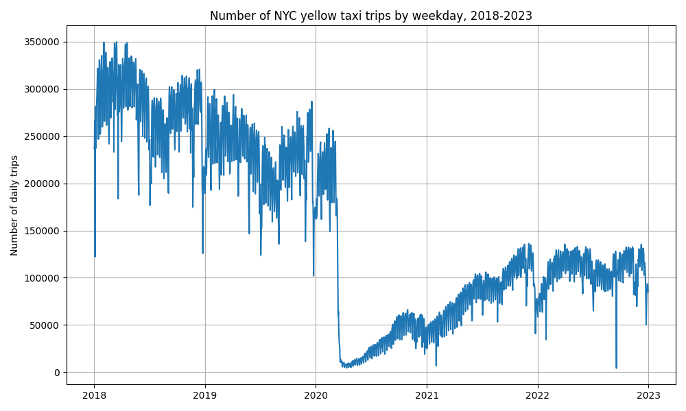
Finally, we want to plot our results. The plot created shows the number of yellow taxi rides per day in NYC. This function runs remotely, on Modal, so we don’t need to install plotting libraries locally.

@app.function()
def plot(dataset) -> bytes:
    import io

    import matplotlib.pyplot as plt

    # Sorting data by date
    dataset.sort(key=lambda x: x[0])

    # Unpacking dates and values
    dates, values = zip(*dataset)

    # Plotting
    plt.figure(figsize=(10, 6))
    plt.plot(dates, values)
    plt.title("Number of NYC yellow taxi trips by weekday, 2018-2023")
    plt.ylabel("Number of daily trips")
    plt.grid(True)
    plt.tight_layout()

    # Saving plot as raw bytes to send back
    buf = io.BytesIO()

    plt.savefig(buf, format="png")

    buf.seek(0)

    return buf.getvalue()

Run everything

The @app.local_entrypoint() defines what happens when we run our Modal program locally. We invoke it from the CLI by calling modal run s3_bucket_mount.py. We first call download_data() and starmap (named because it’s kind of like map(*args)) on tuples of inputs (year, month). This will download, in parallel, all yellow taxi data files into our locally mounted S3 bucket and return a list of Parquet file paths. Then, we call aggregate_data() with map on that list. These files are also read from our S3 bucket. So one function writes files to S3 and the other reads files from S3 in; both run across many files in parallel.

Finally, we call plot to generate the following figure:

Number of NYC yellow taxi trips by weekday, 2018-2023

This program should run in less than 30 seconds.