How we achieved truly serverless GPUs
We are in the age of inference. Billion- to trillion-parameter neural networks are run on specialized accelerators at quadrillions of operations per second to generate media, author software, and fold proteins at massive scale.
Inference workloads are more variable and less predictable than the training workloads that previously dominated. That makes them a natural fit for serverless computing, where applications are defined at a level above the (virtual) machine so that they can be more readily scaled up and down to handle variable load.
But serverless computing only works if new replicas can be spun up quickly — as fast as demand changes, which can be at the scale of seconds. Naïvely spinning up a new instance of, say, SGLang serving a billion-parameter LLM on a B200 can take tens of minutes or stall for hours on GPU availability.
At Modal, we’ve done deep engineering work over the last five years to solve this problem. In this blog post, we walk through what we did.
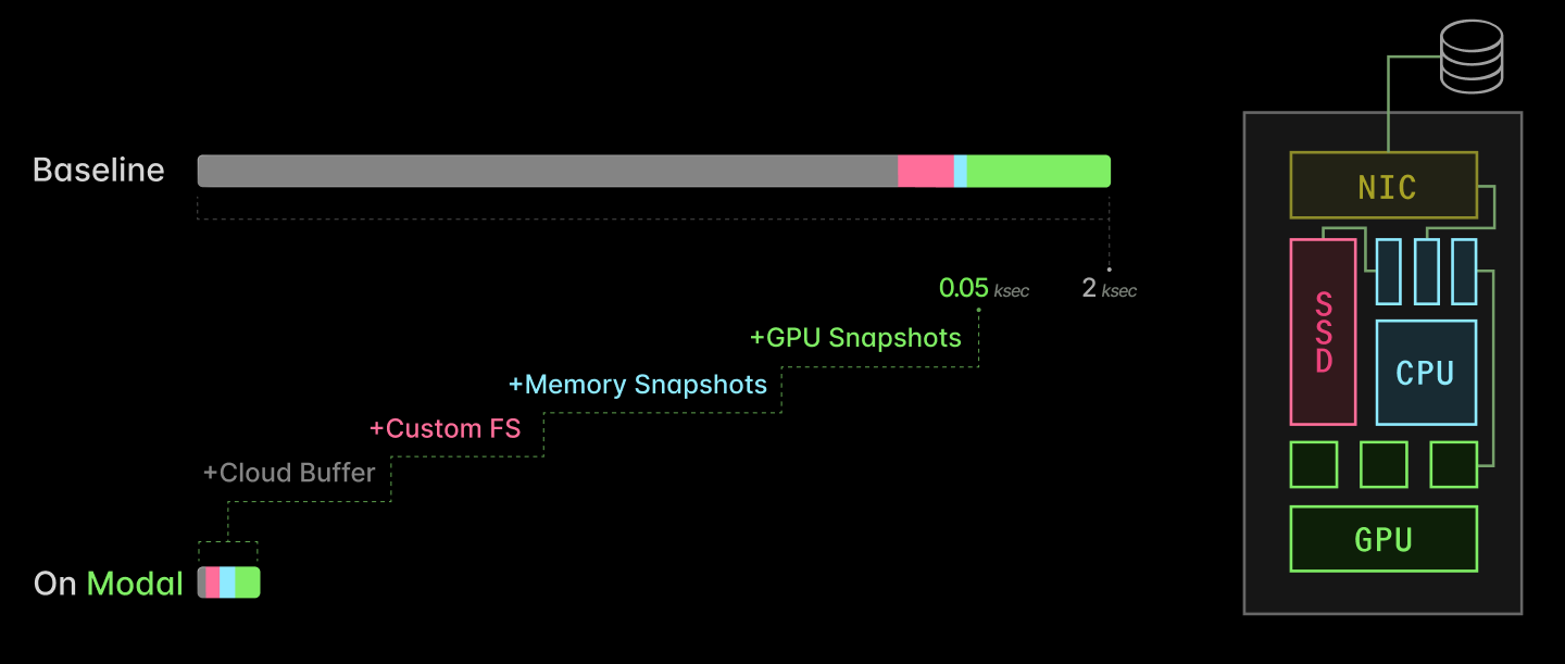
There are four key ingredients:
- Cloud buffers: maintain a small buffer of healthy, idle GPUs to take on new load
- Custom filesystem: serve container images lazily out of a content-addressed, multi-tier cloud-native cache
- Checkpoint/restore: fast-forward through CPU-side initialization by directly restoring processes into memory
- CUDA checkpoint/restore: fast-forward through GPU-side initialization by directly restoring CUDA contexts into memory
Together, they take AI inference server replica scaling from multiple kiloseconds to just tens of seconds.
We’ve shared bits and pieces of this work along the way, because we believe that secrecy is a bad moat. And if more people learn how to use GPUs efficiently, there will be more available in the market for us!
But this blog post represents the first time we’ve put the entire story together in one place. We hope it convinces you that our system is worth buying into — or joining us to build it.
Why care about serverless GPUs? To maximize GPU Allocation Utilization for inference workloads.
First, let’s frame the problem clearly. GPUs are expensive and scarce, so we want to maximize their utilization, where “utilization” is the following unitless quantity:
Utilization := Output achieved ÷ Capacity paid for
There are many ways to measure utilization — to define output and capacity. The most sophisticated and most stringent here is probably “Model FLOP/s Utilization”, which divides raw algorithmic operation requirements by aggregate arithmetic bandwidth.
This is catnip for engineers. It’s also especially critical for “hero run” large-scale training, so it draws a lot of investment and attention, e.g. recently as everyone dunked on xAI’s ~10% MFU.
But at the other end of the stack, there’s a more basic form of utilization that wrecks the relationship between achieved output and allocated capacity for inference workloads, GPU Allocation Utilization:
GPU Allocation Utilization := GPU-seconds running application code ÷ GPU-seconds paid for
Aside on "GPU Utilization" terminology
nvidia-smi and similar tools is in between these two extremes. It reports the fraction of the time that kernel code is running on the GPU — literally, the fraction of time there is a CUDA stream running on the GPU. Read more here.Inference applications have highly variable scale. Unlike training, the demand for capacity is outside the direct control and management of the engineering organization. Instead, it is driven by external user behavior — by markets or social media algorithms or product teams.
Here’s a sample trace of requests per minute from a time-varying Poisson process we use to model inference applications. Notice not only the seasonal variation (daily cycles) but also the long-term trend of increasing variability in demand as the average demand increases.
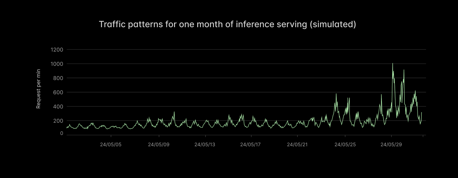
Spiky demand raises serious engineering problems. To borrow from Marc Brooker of AWS: “the cost of a system scales with its (short-term) peak traffic, but for most applications the value the system generates scales with the (long-term) average traffic.” Spiky demand means high peak-to-average ratios, which challenge system economics.
Concretely, imagine the capacity planning for such an application. You might have demand (measured in GPUs required to service requests within latency targets) that looks like this:
With a fixed, over-provisioned GPU allocation, utilization is low
To properly service your anticipated load, you allocate (rack-and-stack, rent on a hyperscaler) 140 GPUs. But most of those GPUs sit idle most of the time — the GPU Allocation Utilization is low.
You might accuse us of talking our book here. But we aren’t the only ones to call this out! See the excellent blog post by Hebbia. And we have data, not just vibes: according to the State of AI Infrastructure at Scale report in 2024, the majority of organizations achieve less than 70% GPU Allocation Utilization when running at peak demand. Actual GPU Allocation Utilizations are commonly often closer to 10-20%.
With fixed allocations, demand can also exceed supply during unanticipated spikes. Trying to anticipate them just increases cost further — more than it increases revenue.
What’s so hard about serverless GPUs? Startup latency.
The immediate solution is to provision auto-scaling capacity: when demand increases, increase your supply.
Done naïvely, this actually worsens the problem:
If allocation is slow, utilization and QoS suffer
Without optimization, going from hyperscaler API request to a running service replica can take tens of minutes.
You need to do the following:
- spin up a new instance and health-check it (minutes to tens of minutes)
- load application program and filesystem state (minutes)
- start the application program on the host, ready it to service requests (tens of seconds)
- start the application program on the device, ready it to service requests (minutes to tens of minutes)
During all of this time, load is in excess of capacity, and QoS typically degrades (absorbed into higher concurrency or queues and thus inflated tail latencies or, worse, 503s). That means angry users. If the capacity takes too long to come online, it can even miss a transient spike. But given the unpredictability of demand and the difficulty of allocation, that capacity typically sticks around, under-utilized, for an extended period.
At Modal, we’ve optimized the spin-up of inference applications on GPUs from many tens of minutes down to a few seconds or tens of seconds. With these optimizations, a wide variety of inference applications of GPUs can run “truly serverlessly”: with provisioned supply tightly matched to system demand.
With fast, automatic allocation, utilization and QoS can both be high
In the rest of this document, we will explain the engineering approach we took and the performance optimizations we implemented for each of the four steps above, which span the stack from cloud storage systems and machine management to local disks, CPUs, and, of course, GPUs.
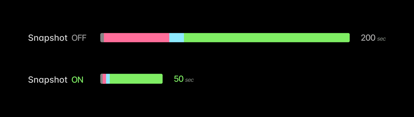
Together, these optimizations allow inference on Modal to spin up 40x faster: 50 seconds instead of 2k.
You can remove tens of minutes of latency by taking instance allocation and health checks out of the hot path.
Consider the first step in replica spin-up:
- spin up a new instance and health-check it (minutes to tens of minutes)
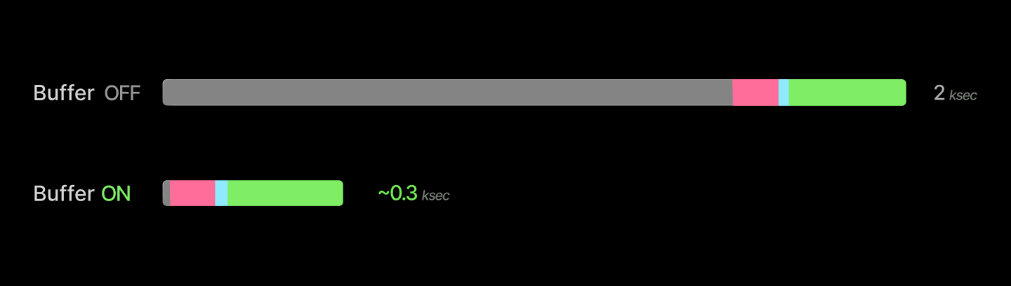
We can remove this from the hot path by doing it ahead of time: running a buffer of idle, healthy GPUs, shared by many applications, scheduling new replicas onto those units, and spinning up new devices into the buffer asynchronously. We can also de-allocate units when the buffer grows too large, as replicas spin down.
Servicing requests from the buffer removes tens of minutes of latency from replica spin-up.
Aside on system- and application-level buffers
buffer_containers. But even then, the size of the buffer you need to absorb spikes of a given magnitude scales with the speed you can create new replicas, and so the optimizations described below are still important for single-workload systems.Managing both active instances and this buffer is a fun linear programming problem, as we’ve written elsewhere. Very roughly, it looks like:

We use Google’s GLOP solver, feeding it scraped prices from cloud providers and tasks from users. Because cloud providers don’t always have capacity at prices and in regions that they advertise, we need to also feed back in the observed supply.

Running a buffer limits the peak allocation utilization below 100%. This is a reasonable trade-off to make, since 100% utilization is generally a mirage. Consider that it is common practice to spin up new replicas and even page engineers when utilization of other resources, like CPU or IOPS, gets too high!
This is important for robustness. A 100% utilized system has no margin for error, and so faults routinely become failures. We can personally recommend adding more buffers to your life — keep an extra toothbrush in your bathroom; keep a charger for your critical devices at home, the office, and on your person.
This buffer is especially useful for accommodating a wider variety of workloads on a single system. At Modal, we’ve leaned into supporting a variety of “development” workloads, not just production serving, because we can quickly create a new development environment. As an extra win, these environments are reproducible-by-default and on prod-ready infra. Closing the gap with production infrastructure also improves development velocity.
The devil is, of course, in the details. One key piece: health checks are critical for GPUs, which fail at a much higher rate than other hardware, including notoriously finicky components like spinning disks. We wrote about our GPU health-checking system in detail here. The tl;dr is that, in our experience, you need to run a short active health check on boot and monitor for health issues that arise later, but you can defer more intense checks (like dcgmi diag) to a slower cadence (for us, weekly).
You can cut container start from minutes to seconds by serving files lazily out of a content-addressed cache.
Now let’s consider the next step:
- load application program and filesystem state (minutes)
In contemporary practice, this generally means booting up one or more containers or VMs.
Roughly, a container is a root filesystem backing a process with limited permissions. For distributed deployments of many containers, performance is bottlenecked by the construction of the root filesystem on the worker instance.
Root filesystems of operating system distros are thicc — tens of thousands of files, gigabytes in size. Naïvely, with a command like docker run, you need to load that whole thing, typically at the few GB/s supported by cloud Ethernet. Even worse, the container image is split into several layers, which must be applied sequentially.
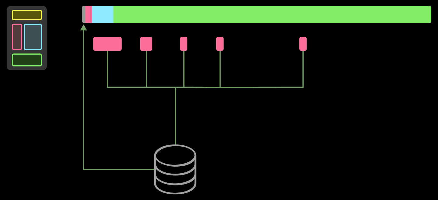
The solution is to disaggregate the container launcher (runc for Docker, runsc for gVisor) from the container image delivery. We use a custom filesystem we call ImageFS, built with libfuse, that combines lazy loading with a multi-tiered, content-addressed cache designed to match cloud provider affordances.
The key “trick” for fast container start that we implement in our custom filesystem is to be lazy, judiciously (as all good engineers do). Container images contain many files, like timezone and locale information for the entire world, that will never be read by most applications. You can skip loading the entire filesystem before the container starts and instead just block start on loading metadata (an index). The metadata is only a few megabytes, so it can be loaded in 100ms or less, along with everything else needed to start a container.
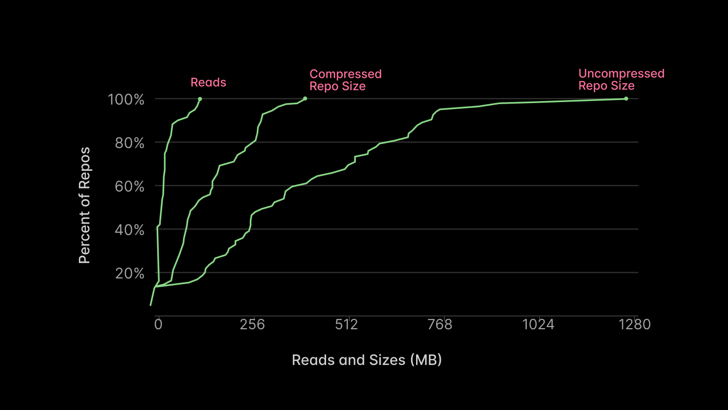
The remainder can be loaded concurrently with other work — or not at all! The majority of the files will not be read, as reported in Figure 5 of the Slacker paper from USENIX FAST ‘16, reproduced below.
We currently implement this filesystem with libfuse. It’s a library for writing Linux filesystems in userspace. The kernel intermediates between one userspace program using standard system calls on files and another implementing a new filesystem (with, in the end, its own syscalls, one of which eventually returns to the original program by way of the kernel). This is much simpler to build and distribute than a custom filesystem in a kernel module.
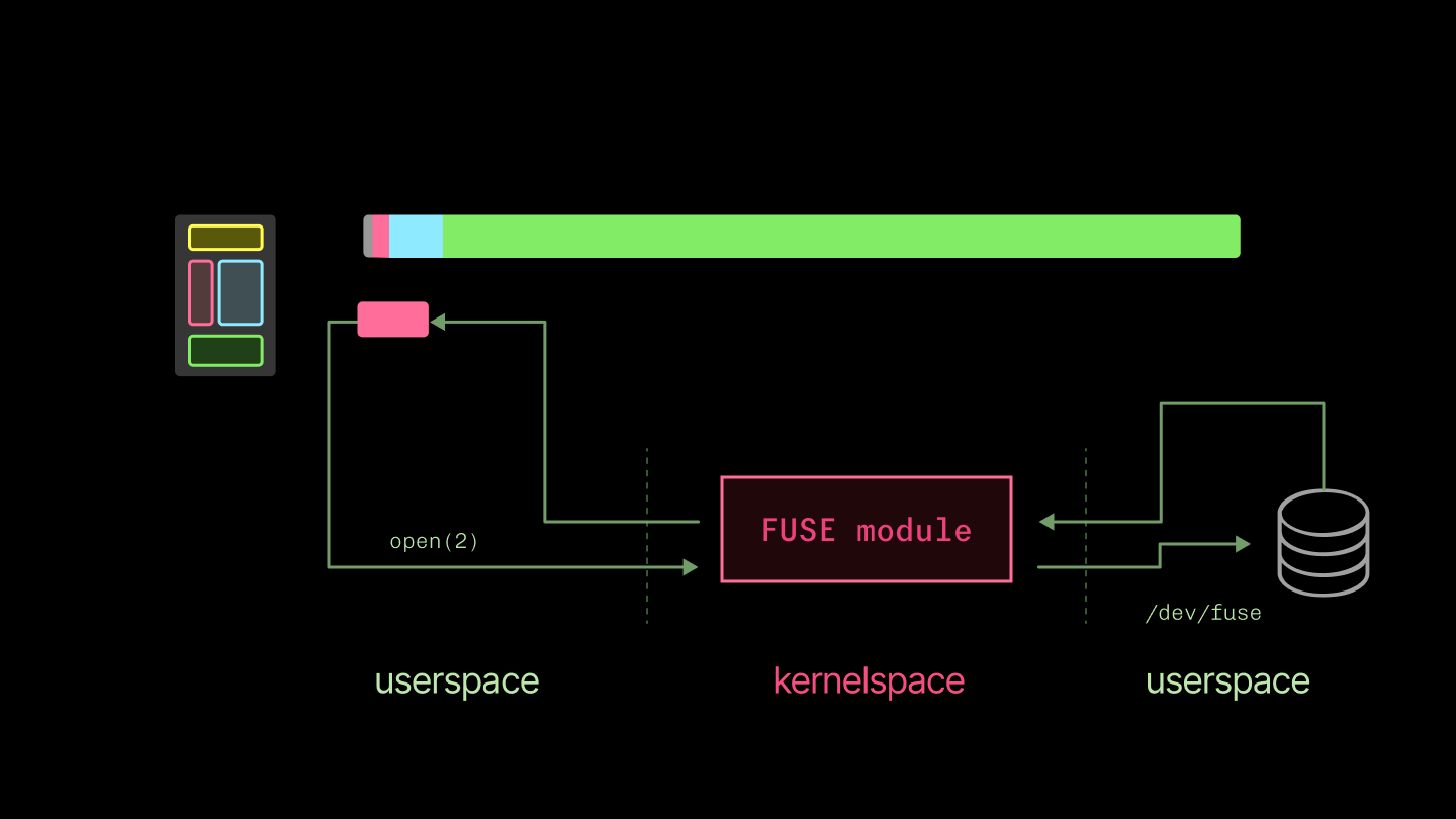
There’s a price: you have double the context switches between userspace and kernelspace. This can be painful for latency-dominated workloads, like reading from a terminal character device, but has less of an impact on throughput-dominated workloads, where we use it. For a useful detailed breakdown of the performance implications, see To FUSE or Not to FUSE from USENIX FAST ‘17.
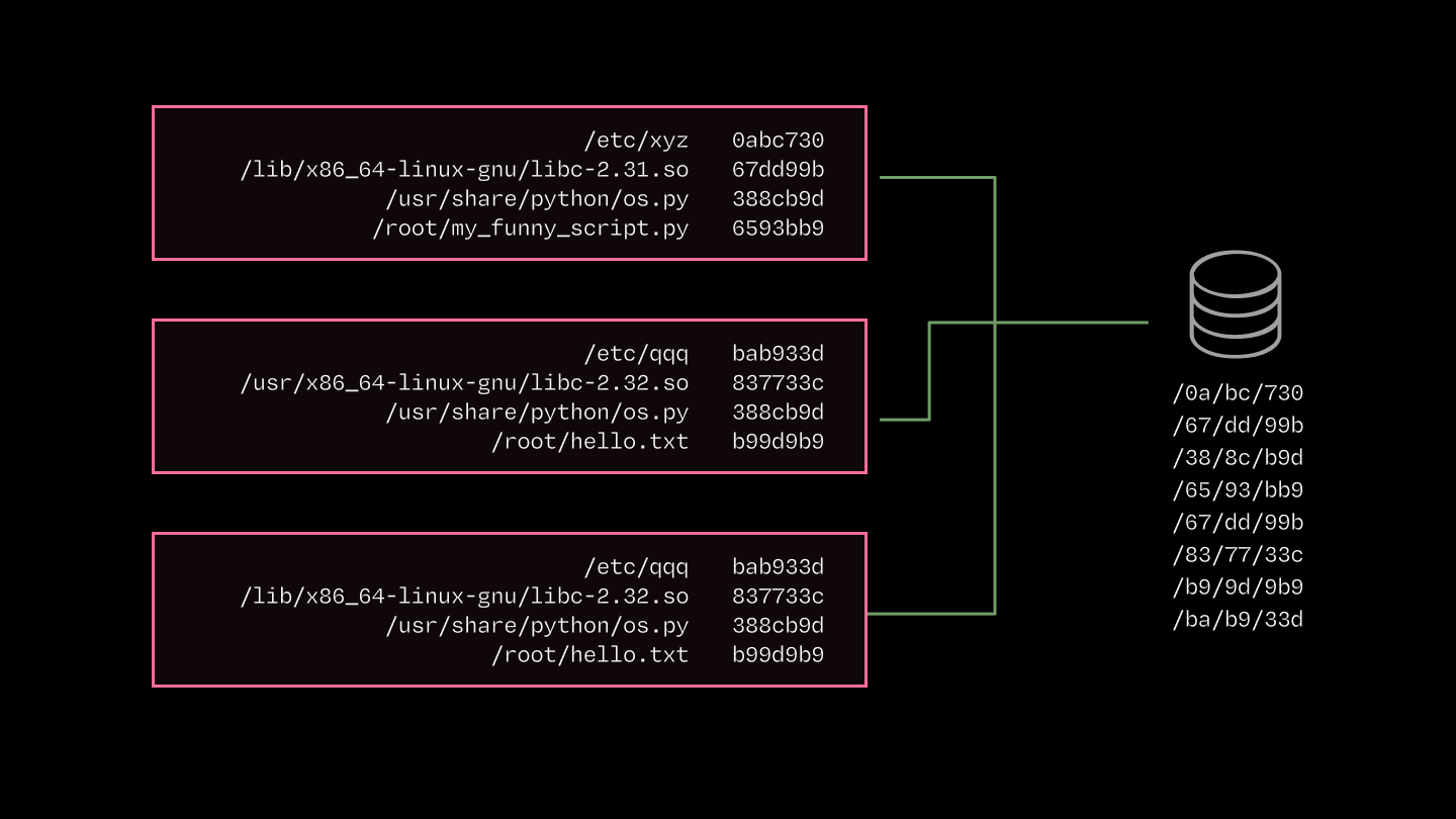
But there’s no free lunch: all the data that is accessed by the container still needs to be loaded. If you naïvely fetched each of the thousands of files accessed by a typical container from object storage, getting from “container start” to torch.cuda.is_available would take hours. So the other key component is a tiered, content-addressed cache that we fill eagerly (but asynchronously).
We use a content-addressed cache because the overlap in image contents across containers is huge. Many inference applications use the same software (e.g. Python, PyTorch, CUDA stack).
But path-based cacheing and Docker’s layerwise cacheing leave performance on the table. For instance, shared bytes aren’t guaranteed to be in the exact same container image layer.
The cache is tiered, just like the caches inside CPUs and GPUs, to map onto the hierarchy of storage available on cloud providers. The diagram and table below list the key components and their throughputs, latencies, & costs.
| System | Read Latency (us) | Read Throughput (GiB/s) |
|---|---|---|
| Page Cache | 0.001 - 0.1 | 10-40 |
| SSD | 100 | 4 |
| AZ Cache Server | 1000 | 10 |
| Regional CDN | 100,000 | 3-10 |
| Blob Storage | 200,000 | 3-10 |
The key breakpoints are:
- Memory: Linux page cache. This is the primary in-memory target. It's your only option for microsecond latencies and has high throughput, but capacity is limited (RAM is expensive, and getting dearer).
- Disk: Local solid state. SSDs are a much gentler step down from memory than spinning disks, but still noticeable. We grab big drives and rapidly fill them up with the most commonly-used content.
- Over-the-network: Blob/object storage. This has essentially infinite capacity — you will run out of money pushing bytes before the hyperscalers run out of money storing them. But it has much higher latency. That latency penalty is punishing, but note that the peak bandwidth can be higher than disk in many cloud configurations!
To really make this rip, you might build more layers between SSD and object storage, like an RDMA layer or within-AZ peer-to-peer sharing. Both are compelling on the numbers, but add a lot of engineering complexity, so we haven’t added them — yet.
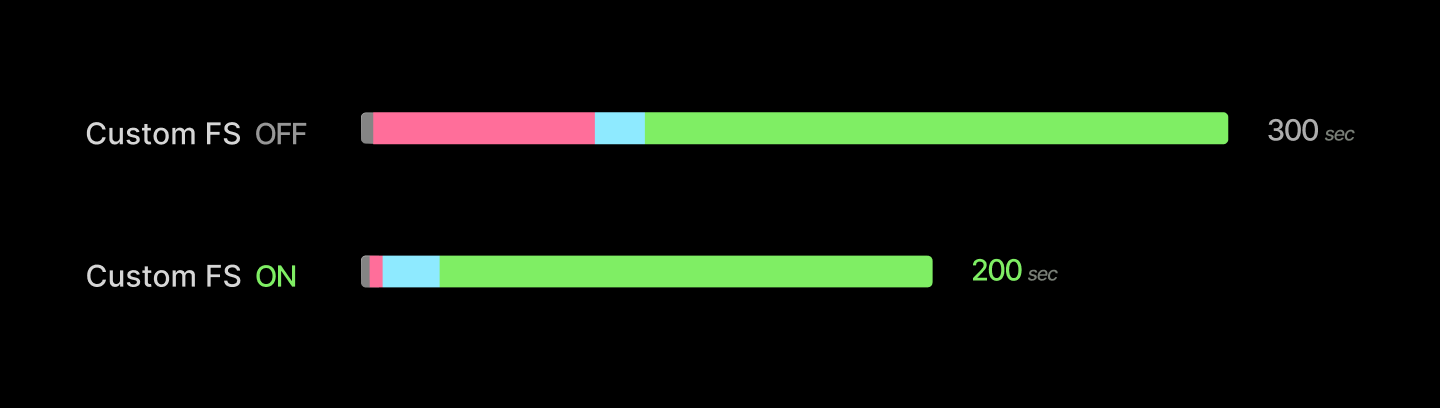
Altogether, we’ve cut container start times down by a minute. For simple applications whose spin-up takes only a few seconds, this is an absolute gamechanger. For heavier applications like an LLM inference server, it removes about a minute from a several-minute start.
The big architectural moves that give integral factors of speedup are followed by a grind of percentage points. We detailed that grind in this blogpost. Here’s a few highlights.
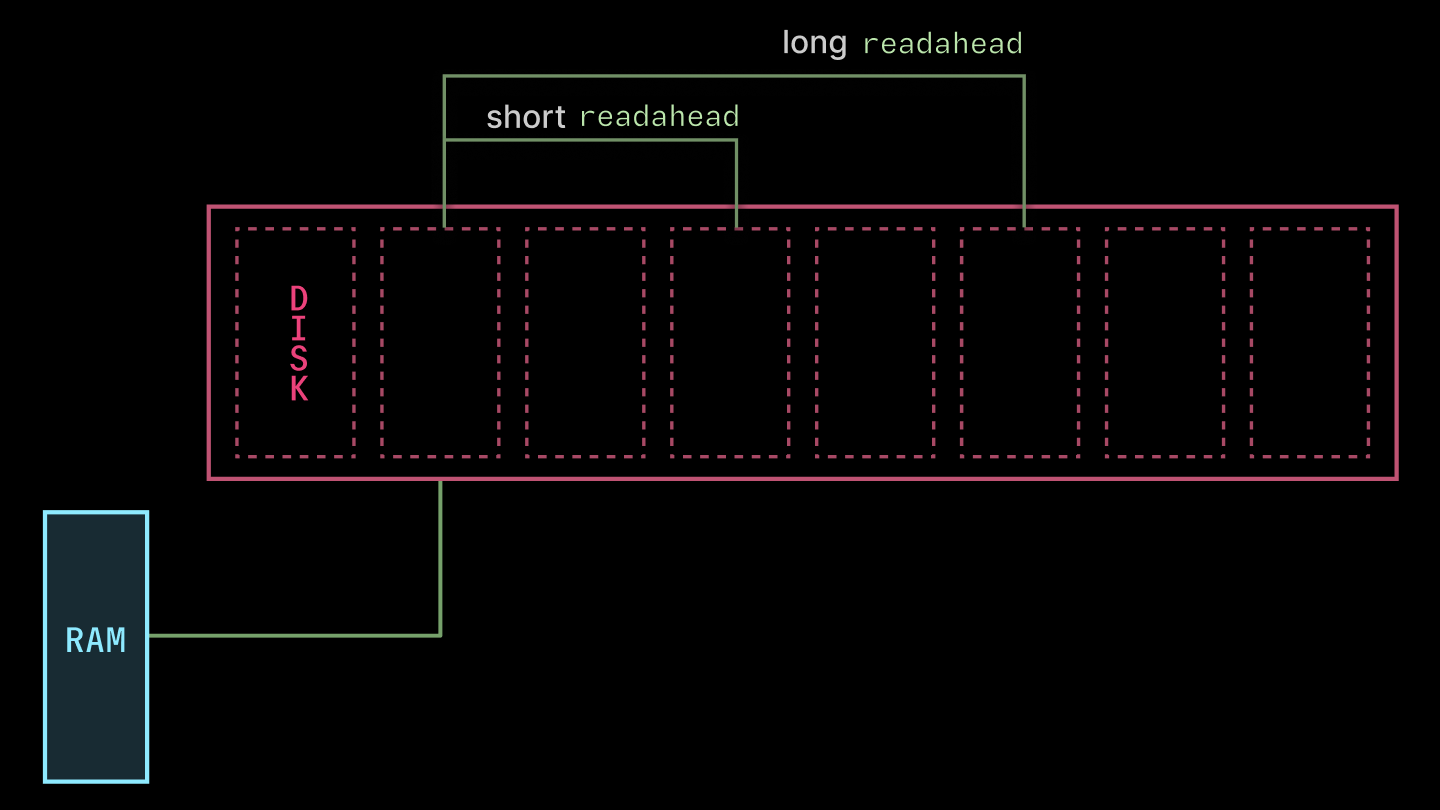
First, libfuse exposes some knobs for performance. We found the most juice from tuning the read_ahead_kb, which directs the kernel to read that many kilobytes ahead of each request (as depicted below). We increased the value from the default 128 to 32 * 1024. The bigger value is nice for the large-read-heaviness of container image loading. Much higher values (in the gigabytes) caused gnarly thrashing.
Second, we skip gzip de/compression of container image layers. DEFLATE is inherently single-threaded (LZ77, Huffman), which limits you to ~100 MB/s, much lower than the throughput of any of the cache layers. If you have full control over container image creation, you might choose to use zstd and pay an upfront cost in image compression to save bandwidth during transfer and avoid bottlenecking the network during decompression. But we also try to keep image creation fast, especially to better support dynamic agent workloads.
You can fast-forward through tens of seconds of application host-side startup with CPU memory snapshotting.
Now, let’s consider our third step:
- start the application program on the host, ready it to service requests (tens of seconds)
This encompasses all of the work that needs to be done to go from the point where the application’s container process is started to the point where the first “useful” work is started — processing the first request.
Consider, for instance, executing the Python statement import torch. This kicks off thousands of lines of Python code that, among other things, executes tens of thousands of syscalls to load a variety of files and interact with drivers. Repeat that for all of the libraries used in a typical inference application, and you’ve got many seconds of work to do between “process start” and “request in-flight”.
The key insight here is that any running process is a heap, some threads, and a file descriptor table. Something like this:
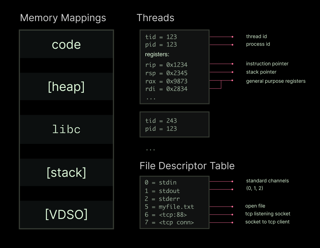
If you can recreate that state (”create a checkpoint”), you can recreate the running process (”restore from checkpoint”). Package that state right, and you can recreate a process from storage faster than you can recreate it by executing a fresh copy.
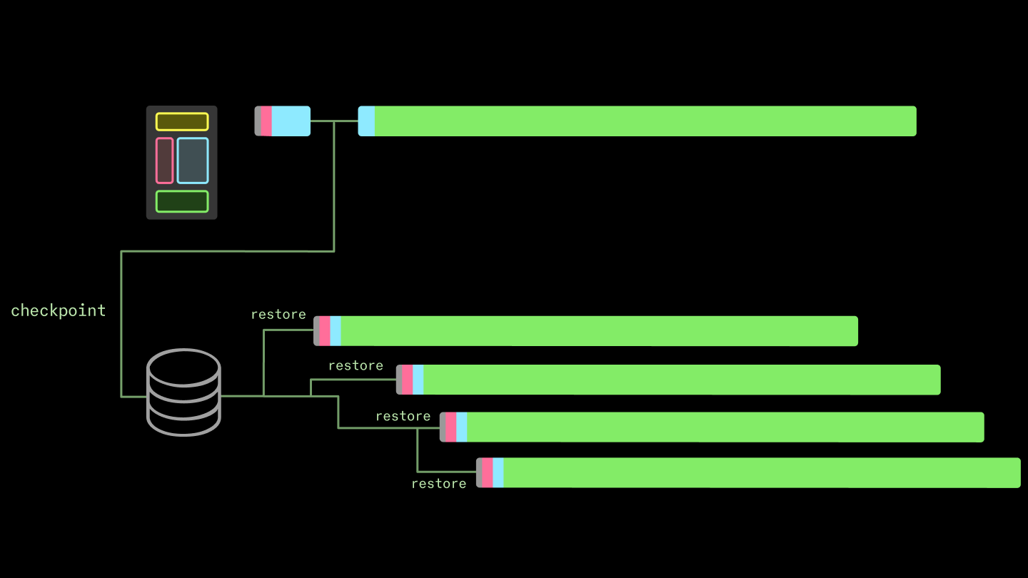
That’s the core idea behind transparent checkpoint/restore interfaces — transparent because user programs do not need to be aware that they are being checkpointed and restored. The implementation of transparent checkpoint/restore in Linux is called Checkpoint/Restore In Userspace (CRIU). Transparent C/R is useful for, among other things, migration of live programs onto different machines. Because our primary goal is to reduce cold start time, transparent checkpoint/restore is not a requirement in our system.
So we expose the C/R interface to users via our container lifecycle management interface. It looks something like this:
@app.cls(enable_memory_snapshot=True) # checkpoint global scope
class InferenceService:
@modal.enter(snap=True) # checkpoint when this method returns
def startup(self):
...
@modal.enter(snap=False) # run in container init, but don't checkpoint
def finalize(self):
...
@modal.method() # run with each invocation
def run(self, messages):
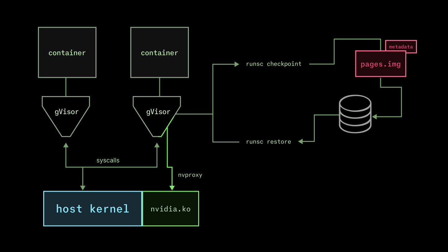
...We don’t use Linux C/R currently. We run user containers with gVisor’s runsc, which effectively emulates (a subset of) the Linux kernel in userspace. This limited surface area provides automatic protection from exploits like the recently-identified CVE-2026-31431, bka “CopyFail”. We’re particularly interested in (and contribute to!) the nvproxy sub-component, which communicates with the GPU’s kernel-mode drivers.
Because applications only interface with this emulated kernel, they can be checkpointed and restored by it without cooperation from the host kernel.
Checkpoint/restore is actually especially easy for runsc. A container in the runsc runtime is straightforwardly a state machine. That is, the runtime is architected (in Go) as a collection of tasks with cooperative preemption, as in most other systems with async/await-style concurrency. The system is already being interrupted and then continued at every await point, so it’s “only” a matter of serializing that state into a checkpoint.
More precisely, the runsc checkpoint command stops a container and produces state on disk that can be used to restart the container with runsc restore (docs here). By default, it’s a zipped archive, but we generate without compression (remember the gzip bottleneck!). The key file is pages.img, which contains the raw page data. It is at least 100 MB but can be many GB (though generally not larger than system memory).
There’s a lot of other moving pieces, but checkpoint restoration performance is won and lost on how quickly this can be brought into the host page cache. We use the same custom filesystem machinery described above to deliver the checkpoint files.
The result is about a 10x reduction in time to load the host-side components of a new replica. You can read more about our memory snapshotting system in this blog post.
import torch
Stable Diffusion
There are some limitations here. Checkpoints are very sensitive to the details of the host environment. For example, the AWS g6.12xlarge instance type does not support the pclmulqdq Perform a Carry-Less Multiplication of Quadword instruction and so it cannot accept any snapshot created on a host which does — that instruction might be hard-coded into a code region page, and issuing it would lead to an illegal instruction fault (or worse). So on a heterogeneous cloud platform like Modal, which aggregates capacity from many providers to ensure low costs and high availability, a single inference server deployment needs more than one snapshot.
Second, this system only considers the host-side state of the program. But among the file descriptors in a process’s state might be a handle on the GPU via the drivers, and the program state properly includes whatever state is on the device. This is where the lion’s share of time is spent when starting up an inference server, so the wins from pure host-side checkpoint/restore are limited. But they unlock device snapshotting, where we turn next.
You can fast-forward through minutes of application device startup with GPU memory snapshotting.
Now, let’s consider the final step in creating a new inference server replica:
- start the application program on the device, ready it to service requests (minutes to tens of minutes)
There are two distinct pieces of work that can both take many minutes for a contemporary inference workload. First, the neural network weights need to be loaded from storage into the GPU memory. Second, the code around the neural network (the “inference engine”) needs to do some setup work.
Frontier LLM weights these days run from the billions to trillions of bytes (aka, GB to TB). We use the same basic storage affordances as in the custom filesystem to load model weights, and so model weights are loaded at a few gigabytes per second. That’s a total latency between a few seconds and a few hundred seconds. Checkpoint/restore doesn’t help you here, since you are bottlenecked on throughput for large reads, not work that is readily skippable via snapshotting.
Aside on weight loading
But weight loading is not the only device-dependent slow step. Inference engine setup involves multiple compute-heavy, device-dependent steps that produce small in-memory artifacts that are tricky to cache. For instance, the vLLM inference server captures CUDA graphs and runs the Torch compiler. Each of these steps takes between tens of seconds and minutes. CUDA graphs are made up of pointers to tensors and kernels and have no native serialization option. The Torch compiler can produce serializable artifacts. But in our experience, validating cache hits on these artifacts is often slow (seconds to tens of seconds), limiting the benefit of cacheing.
These small, in-memory runtime artifacts that are expensive to produce make inference setup a prime candidate for checkpoint/restore. However, checkpointing based on runsc or CRIU only operates on host memory, not device memory. Even though most of the inference engine artifacts are host-side, the setup process creates device resources that must be checkpointed and restored.
Nvidia’s recent driver versions include an elegant solution to this problem. In short, the driver checkpoints device memory in host memory so that it can be checkpointed to disk by a host-side checkpointing system. Then, once the host-side system has restored the host memory, including the device checkpoint, the driver restores the device memory.
The device checkpoint/restore builds on the host checkpoint/restore, which builds on the underlying filesystem. Infrastructure compounds.
The results are striking: typical speedups are between 4-10x, reducing container start time from several minutes to tens of seconds.
There are a few caveats to this, which we document here. First, snapshotting of multi-GPU programs is tricky, since nccl programs are not designed for pauses and frequently deadlock when one peer goes quiet. Second, while our experience has been that almost any application can be snapshot, most applications require some minor adjustment first. For instance, snapshotting vLLM or SGLang works best with weight offloading — moving the weights back onto the host before checkpointing. Additionally, the engines generally eagerly create an (empty) KV cache, which can be recreated much more quickly than it can be restored from a checkpoint.
With these adjustments in place, LLM inference server replicas can boot up nearly an order of magnitude faster with snapshots. Below, we report the latency cumulative distribution functions for fresh replicas of vLLM or SGLang serving a ~1 GiB language model (Qwen 3 0.6B in bf16). This includes all latency to create new replicas on Modal — any queueing for machines, container start, host- and device-side prep. Across over ten thousand cold starts, we observed superior latency at every quantile for the snapshot deployments.
Boot 1 GiB model in vLLM
Boot 1 GiB model in SGLang
Averages improve as well.
| Snapshot OFF | Snapshot ON | |
|---|---|---|
| vLLM boot latency (mean) | 95,679 ms | 13,797 ms |
| SGLang boot latency (mean) | 83,713 ms | 17,486 ms |
You can read more about GPU snapshotting, including additional benchmark results, in this blog post.
We have run this stack at the scale of tens of millions of replicas across many use cases.
Usage numbers for the last three months, February - April of 2026, appear below.
| Replicas restored | Hours of execution | Distinct snapshots created | |
|---|---|---|---|
| CPU Snapshots | ~35,000,000 | >5,000,000 | ~1,000,000 |
| CPU+GPU Snapshots | ~15,000,000 | >2,000,000 | ~700,000 |
CPU and GPU snapshots are used by a few hundred distinct organizations across a variety of use cases.
CPU snapshots are most commonly used in data pipelines or job queue systems, but they are also frequently used across a variety of use cases to speed up initialization, especially Python imports.
GPU snapshots are also used across a variety of domains. Because of the current restriction to a single GPU, they are most commonly used for models with sizes in the few to few tens of gigabytes. That includes the smaller end of large language/vision-language models, used for structured data extraction or for tasks with low cognitive complexity. We have found that GPU snapshots are also popular for audio/voice use cases, both for speech-to-text/automated speech recognition and text-to-speech/voice generation.
Spotlight Use Case: Reducto scales document processing seamlessly up to thousands of GPUs.
Reducto is a document processing platform that uses vision-language foundation models to extract structured data from unstructured documents. You may have read about their contributions to the JMail project, for which they indexed the correspondence of international criminal Jeffrey Epstein.
One of the primary constraints on Reducto’s document processing system is a high peak-to-average ratio. A customer may appear at any moment with a request to process, say, an entire enterprise’s collection of Notion documents. These jobs have deadlines on the scale of tens of minutes, which can only be met by horizontally scaling across hundreds or thousands of GPUs.
Fast container starts allow Reducto to hit these deadlines without maintaining idle capacity — to run a kilo-GPU inference workload “truly serverlessly”.
In particular, the addition of GPU memory snapshotting pushed down cold starts about six-fold, from ~70s to ~12s.
You can read more about Reducto’s use of serverless GPUs for inference on our blog.
Coda
The existing container stack and cloud services built with it are designed for a previous generation of workloads, like hosting websites and interacting with databases. They aren’t designed for training or inference, and this impedance mismatch is a tax on cost, efficiency, and performance for teams building inference applications.
We built Modal to bring cloud infrastructure up to speed (literally) with the demands of artificial intelligence. We’re sharing how we did it for a few reasons.
First, we hope you’re as excited about building applications on this infrastructure as our customers, like Physical Intelligence, Runway, Ramp, Zencastr, Lovable, Substack, and Suno. You can start using it, including $30 of free usage credits per month, right now.
Second, we built this system on top of and with reference to a number of excellent open source or well-documented systems, from Linux CRIU to AWS Lambda. We want to pay that forward. If you take inspiration from our work, we’d love to hear about it.
Finally, we’ve still got a lot of work to do — those RDMA networks don’t configure themselves! We hope that sharing what that work looks like will get more of the best engineers interested in doing it with us. “Building a boat isn’t about weaving canvas, forging nails, or reading the sky. It’s about giving a shared taste for the sea.” Shipbuilders and sea-yearners, inquire within and share your favorite story of working for hours to save a millisecond, one trillion times.
The authors would like to thank Vikram Mailthody, Steven Gurfinkel, Stephen Jones, Radostin Stoyanov, Rodrigo Bruno, and Jordan Sassoon for their input.