Transcribe speech 100x faster and 100x cheaper with open models
Open ASR models have arrived.
Since ChatGPT showed the world that generative modeling and artificial intelligence are ready for industrial-scale commercial applications, the most performant modeling and intelligence services have largely been provided by proprietary APIs.
But over the past year, open weights models have caught up across a range of domains from language to images to video. Open source frameworks to run those models, like PyTorch and vLLM, have kept pace.
And you might have missed it, but in just the past few months, there’s been a wave of highly performant open weights models focused on automated speech recognition (ASR), aka speech-to-text (STT), aka transcription.
These models - which include NVIDIA’s Parakeet & Canary and Kyutai’s STT - report incredible accuracy (word-error rate, WER), speed (real-time factor, RTFx), and include additional features like multiple languages, word-level timestamps, or vocal activity detection (VAD).
| Model | ESB WER, English (%) | RTFx | Languages | Timestamps | VAD |
|---|---|---|---|---|---|
| nvidia/parakeet-tdt-0.6b-v2 | 6.05 | 3386.02 | ✅ | ✅ | ❌ |
| nvidia/canary-1b-flash | 6.35 | 1045.75 | ✅✅✅✅ | ✅ | ❌ |
| kyutai/stt-2.6b-en | 6.4 | 88.37 | ✅ | ✅ | ✅ |
Some CEO math: Modal + Open ASR > 100x
A quick back-of-the-envelope calculation was enough to get us pretty excited about these new models.
- Proprietary APIs charge about 0.4¢ per minute of audio
- The Open ASR leaderboard indicates an RTFx, aka audio minutes per wall clock minute, of several thousand on A100s
- An A100 or L40S GPU on Modal is currently about 4¢ per minute
Even making pessimistic assumptions about overhead, the napkin math indicates it should be possible to hit 100x cheaper per minute of audio when running transcription.
We heard some rumors this was true (from people churning off proprietary APIs and onto our platform), so we decided to see for ourselves.
We
- implemented a batch transcription service on Modal
- using NVIDIA’s parakeet-tdt-0.6b-v2 (English) and canary-1b-flash (multilingual)
- and compared it to a popular proprietary API
- on roughly a week (7 * 24 hours) of speech data from the ESB benchmarking datasets used in the HuggingFace ASR Leaderboard.
A few optimizations and experiments later and we were able to deploy a transcription service that is over 100x faster or 100x cheaper than the proprietary API we tested while matching its error rate. (Technically, the open models had a slightly lower error-rate on this dataset…)
That’s
- one week of audio
- transcribed in just one minute
- for just $1.

| Relative ETE Throughput | Cost Savings | |
|---|---|---|
| English only | ||
| Parakeet, Fastest | 112x | 60x |
| Parakeet, Cheapest | 25x | 200x |
| Proprietary API | 1x | 1x |
| Multilingual | ||
| Canary, Fastest | 80x | 55x |
| Canary, Cheapest | 12x | 152x |
| Proprietary API | 1x | 1x |
How we transcribed a week of audio in a minute for a dollar.
We want to share some of the details of our implementation and optimization process related to batching and distributing transcription requests across workers.
Hopefully these can help you optimize your own transcription service and build more performant Modal apps.
The real world use case: transcribing many hours of audio per hour.
Before we jump into the engineering, let’s make sure we’re clear on the use cases we’re trying to optimize the system for. A good idea for any performance engineering task!
The ideal use case for large-scale batch transcription is a company that’s collecting many, many seconds of audio per second. Say a call center where your call may be recorded for quality assurance, generating thousands of hours of new recordings every hour. The data is dumped on S3 loaded into a data lake and every hour we need to load up the new files and transcribe them.
Or you might be a foundation model company that’s looking for language tokens wherever you can find them. You’ve scraped audio files from all over the Internet and want to transcribe them so that they can be used for next-token-prediction training of a text-based language model.
In both cases, we can assume that at rest, the data lives in some object/file-like cloud storage, and the figures of merit are
- how quickly we can finish processing all of the data
- how much the processing costs
Batch transcription is qualitatively different from a streaming scenario where we have many users who each require a low-latency transcription service for real-time applications. The two are evaluated with different metrics and require different implementation choices.
If you’re interested in streaming transcription, check out our Kyutai STT example. For use cases somewhere between pure batch jobs and streaming, you might consider dynamically batched transcription (code sample here).
Designing a benchmark for batch audio transcription
We sanity-checked quality via WER and the ESB/HuggingFace Open ASR Leaderboard benchmark.
One advantage of choosing models included in the HuggingFace ASR Leaderboard is that we can use the same datasets and WER scoring code. This allows us to verify our deployments haven’t introduced any bugs or somehow reduced accuracy.
It also helps ground our accuracy comparison to the proprietary API in the full leaderboard results.
But we measured end-to-end performance, not just model execution time.
ASR models report speed as RTFx which only considers transcription time. This makes sense if you’re running inference locally (relative to the audio byte producer and the text consumer). But for distributed cloud services, you need to consider data transfer times. For a cloud service with horizontal scaling, you also need to consider cold start times.
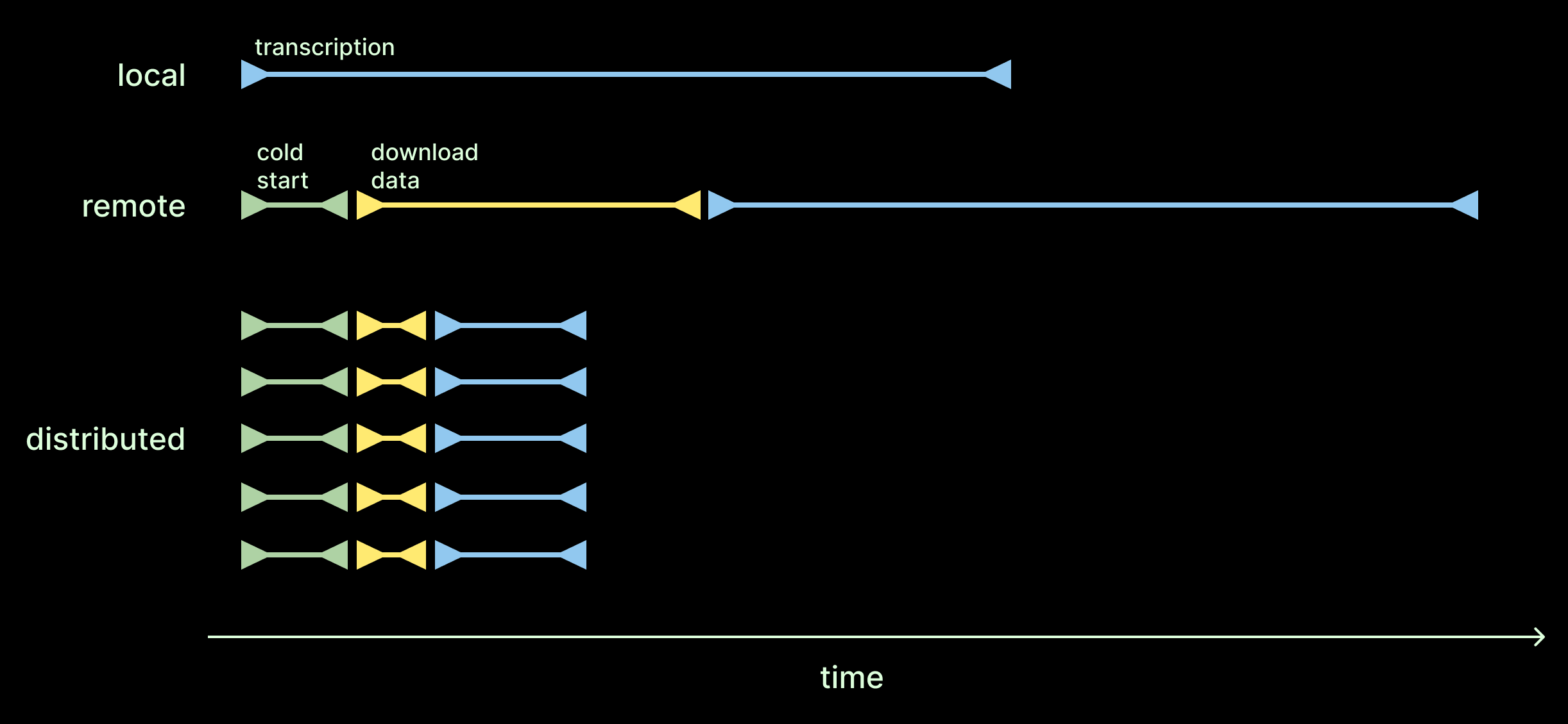
We get why model providers want to focus on the time the model takes. But to us, it seems unfair to ignore these parts of the process. Most of us ultimately care about the total time our jobs take, not just the fancy “AI” part. To account for this, we report end-to-end throughput which measures the duration at the client and includes cold-starts, network latencies, and other forms of data movement.
Architecting batch transcription with Modal
We used Modal to set up batch processing of transcription using both open weights models and a proprietary API. And in both cases we spent time optimizing throughput.
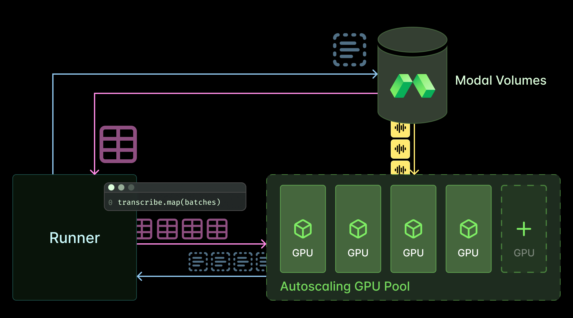
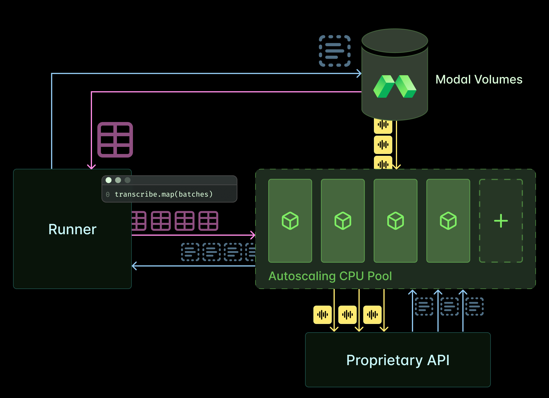
The main difference between the two architectures is that we provision GPUs and perform transcription on the Modal container itself when using open models whereas we provision CPU containers which make parallel HTTP requests when using the proprietary API. We don’t include the costs of CPUs in any of our numbers. Compared to GPUs and API requests, they might as well be free!
Deploying NVIDIA’s ASR models on Modal GPUs
NVIDIA lays claim to many of the most accurate and fastest open ASR models. We opted to use their parakeet-tdt-0.6b-v2 model, since it reports 3x faster inference than any model with a comparable error rate, as well as its sister model, canary-1b-flash, which has a lower RTFx but handles multiple languages (English, Français, Español, und Deutsch).
We built our service on NVIDIA’s NeMo framework, which makes it relatively simple to switch between any of NVIDIA’s ASR models.
It was a pretty small lift to take the NeMo code from the HuggingFace Open ASR GitHub repo and turn it into a distributed batch service that will dynamically provision GPUs when we spin up a job. A basic demo fits in a single Python file — no YAML, no problems.
Saturating a proprietary API from Modal CPUs
We selected a popular and competitive proprietary ASR API and tested the base level of service. To provide a fair comparison on throughput, we tested multiple approaches to saturate request rates using a distributed Modal deployment. The core strategy to maximize throughput was to distribute the transcription requests over a number of workers equal to maximum concurrency limit of the API.
We observed throttling but we ignored it to be more fair.
Our request throughput was potentially throttled during runs over full the dataset. To be as fair as possible, we report the maximum throughput we observed. While we can’t be sure we are measuring the same thing, our estimated maximum throughput matched the rate reported on the API’s documentation and marketing site.
Doing some 100x engineering
Distributing a computation - whether it’s across the streaming multiprocessors in a single GPU or across a global fleet of cloud instances - can result in impressive throughput gains. But it can alternatively result in a reduction in throughput depending on how effectively your implementation moves data around and makes use of the available hardware.
Determining the best implementation is a combination of thoughtful design when architecting the system and experimentation with the systems knobs — you know, “engineering”.
Distributing data into batches
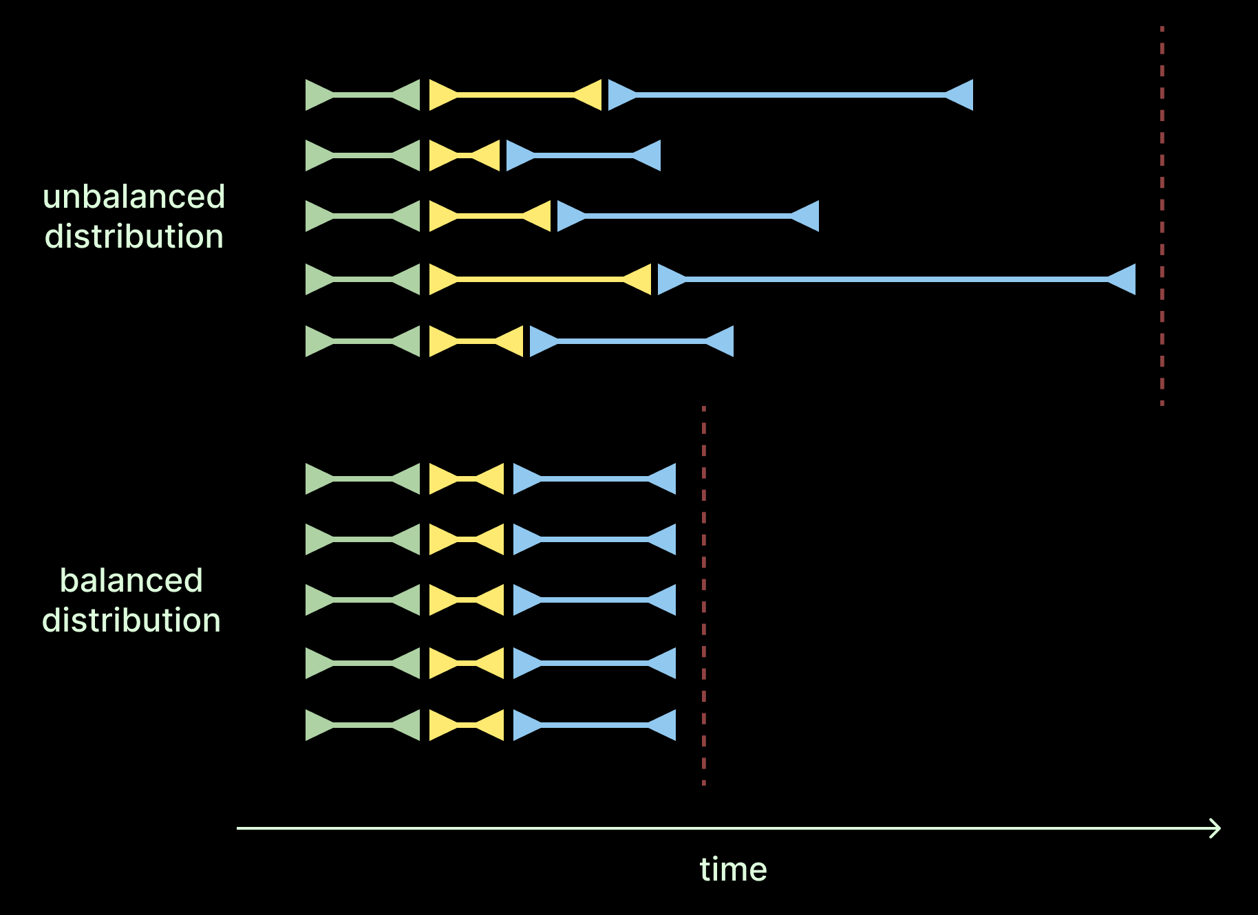
We can think about some of our optimizations as packing problems - both in terms of memory and time. When we don’t pack memory efficiently we end up performing more iterations or requests than is necessary. When we don’t pack time efficiently, we end up waiting on work while also having empty compute lanes. This is the difference between a balanced and unbalanced load distribution.
In other words, we want to fill all of the available lanes all of the time.
In our system, we need to distribute data into batches over requests to our Modal Function as well as within each GPU.
Batching audio files into requests
To balance the workload across our Modal autoscaling pool, we want to match the distribution of data sent in each request in the following ways
- the number of bytes
- the number of audio files
- total duration of audio files to ensure that each worker spends about the same amount of time downloading data as well as performing transcription.
Fortunately, for large batch jobs we can simply shuffle the data before dealing it into request batches to ensure the distributions are matched. Be sure not to skip this step. There can be correlations between sample ordering and duration baked into your tables; or the data may come pre-sorted as is the case with the ESB/HF datasets.
Batching bytes to make GPUs go brrrt
Most, if not all, of the entrants on the ASR Leaderboard perform GPU inference in batches. For Parakeet this is as simple as adding the batch_size keyword argument to the transcribe call.
Batch inference makes better use of the GPU, a massively parallel, throughput-oriented computing device. It exposes more parallelism to the underlying program runtime and hardware. Our batch size is limited by the GPU’s memory.
Luckily, the NVIDIA submissions to the HuggingFace leaderboard give us some idea of what GPU batch size to use. And during experiments we found that a range of values performed more or less equally well.
But what about packing in time?
Longer recordings take longer to process. This has important consequences for how we distribute audio into batches because a batch is only complete when all of its elements have been processed. This leads to a strategy of matching audio duration within GPU batches to maximize execution time within each lane of the GPU.
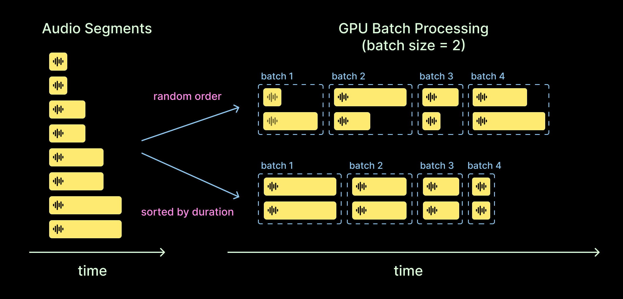
To implement this strategy, sort your audio segments before mapping your inference calls. Remember, we’re talking about sorting the audio for a single GPU worker/request. We shuffled before batching into requests to balance the workload, but now we want to sort each of those requests to maximize the efficiency of GPU batching.
If you are getting PTSD flashbacks to sort phases in Hadoop Map-Reduce, 1) we feel you and 2) we’re hiring and we promise you won’t ever see HDFS in prod. While the fix itself is relatively simple, the effect can be quite large, as recording lengths are often exponentially distributed (presumably reflecting underlying memoryless dynamics).
Downloading data to workers
We also need to move the data to each worker. And the best solution is highly dependent on the location and state of your data at rest.
In our setup, we start with audio segments saved as WAV files on a Modal Volume. Before transcription begins, we download the files to local disk. To minimize transfer time, we use Python’s multiprocessing.ThreadPool to saturate the network bandwidth with parallel requests. Avoiding disk writes by keeping files in memory might speed things up a bit, but SSD throughput is so much higher than network throughput that we didn’t think it worth trying.
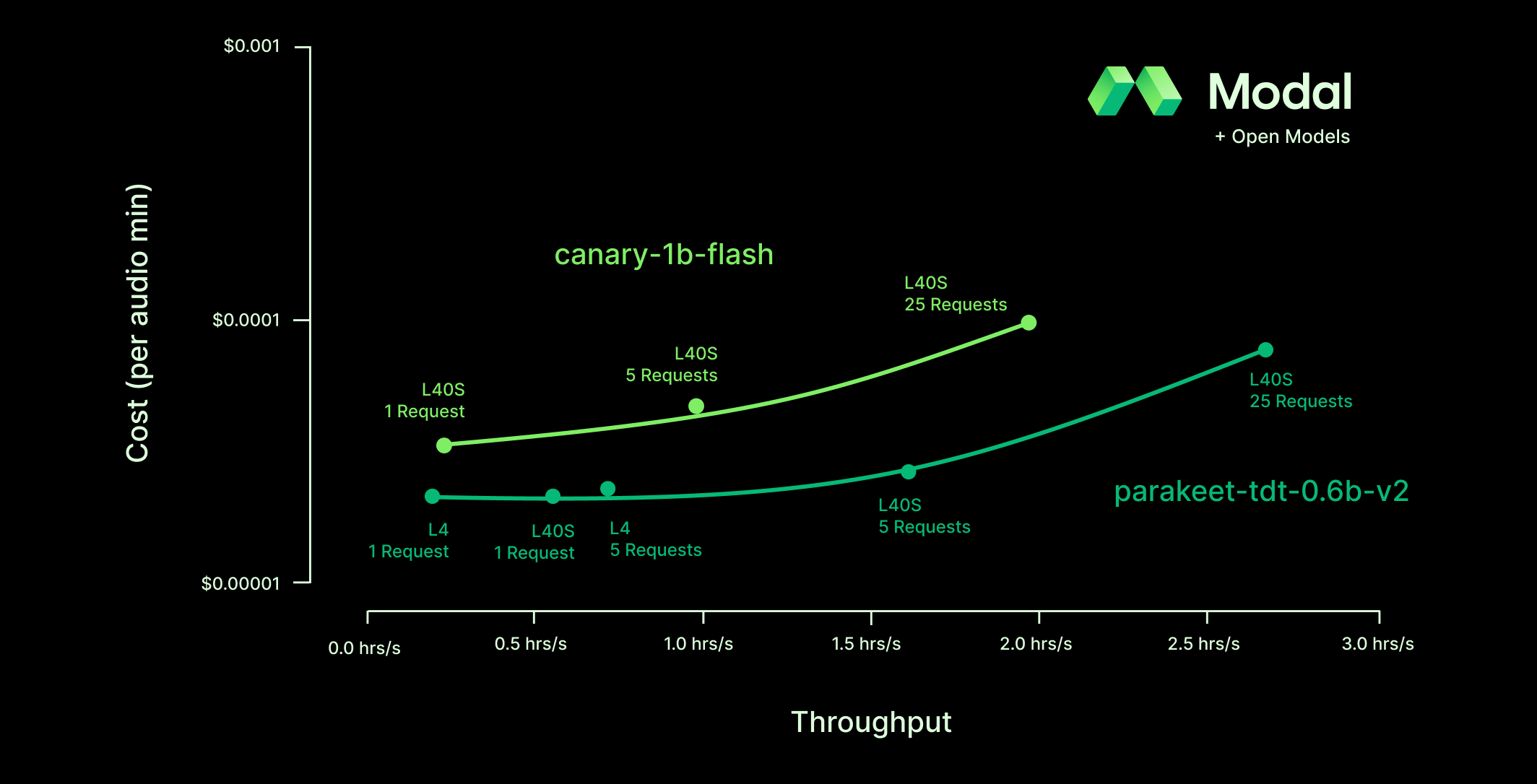
Selecting a GPU type and number of requests
There are two more design decisions that will have a large impact on our cost and throughput: GPU model and number of requests.
These choices interact with each other in somewhat complex ways: for instance, big GPUs are faster but more expensive. Instead of trying to reason through which combination will lead to the best results, we chose to empirically determine the optimal configurations - MLEs in the audience, think hyperparameter fine-tuning.
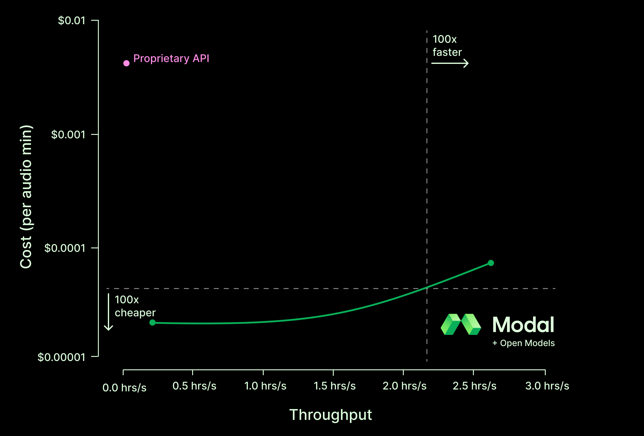
Because we have two figures of merit, cost and throughput, there is not necessarily a single “optimal configuration”. There is instead a Pareto frontier of configurations (per model) that dominate over all others but represent distinct trade-offs of cost and speed.
Note that the proprietary inference service is not shown on this chart — if we were to draw it, it’d be somewhere near the word “proprietary” at the beginning of this sentence.
For our batch transcription service, we can choose different combinations of GPU model and number of workers depending on whether we want to save money or save time or maybe split the difference. But regardless of exactly which configuration we choose, deploying the top open ASR models on Modal is competitive alternative to proprietary services.
Run your own large-scale, high-performance audio transcription on Modal in minutes!
Modal users like Substack and Zencastr run their transcription workloads at scale on Modal — no proprietary APIs or AWS YAML Engineer certifications needed, just open source models, a Python file or two, and a Modal API key to provision the resources on our platform.
Learn more about boosting your audio inference services with Modal, quickly deploy your own batch transcription service using the code from this post, or check out our other speech-to-text examples.