The era of “get your AI from an API” is rapidly coming to a close.

High-quality open weights models and high-performance open source software together mean that you can easily run your own API to generate images or music or text, with all the control and customization self-hosting affords.

But having the ability to run your own generative inference raises a bunch of questions: when does it make sense, how do you do it, and, importantly, how do you do it with the same performance and quality that proprietary generative APIs provide?

We recently shared our results and recommendations for running your own LLM inference. But we also like media generative models, and optimizations look quite different. Where LLM inference is all about finding the right high-level framework and tuning the knobs, diffusion-based models of images require getting a lot closer to the metal.

In this blog post, we walk through how we made running the popular FLUX.1-dev model by Black Forest Labs as an autoscaling service on Modal competitive with proprietary providers on speed and price by running the inference three times faster and speeding up cold boots. You can find the code here.

tl;dr: 1.5x from optimizing compiler and hardware awareness, 2x from approximate caching

We determined that in order to be competitive with APIs serving FLUX.1-dev images, we needed to return results in under three seconds.

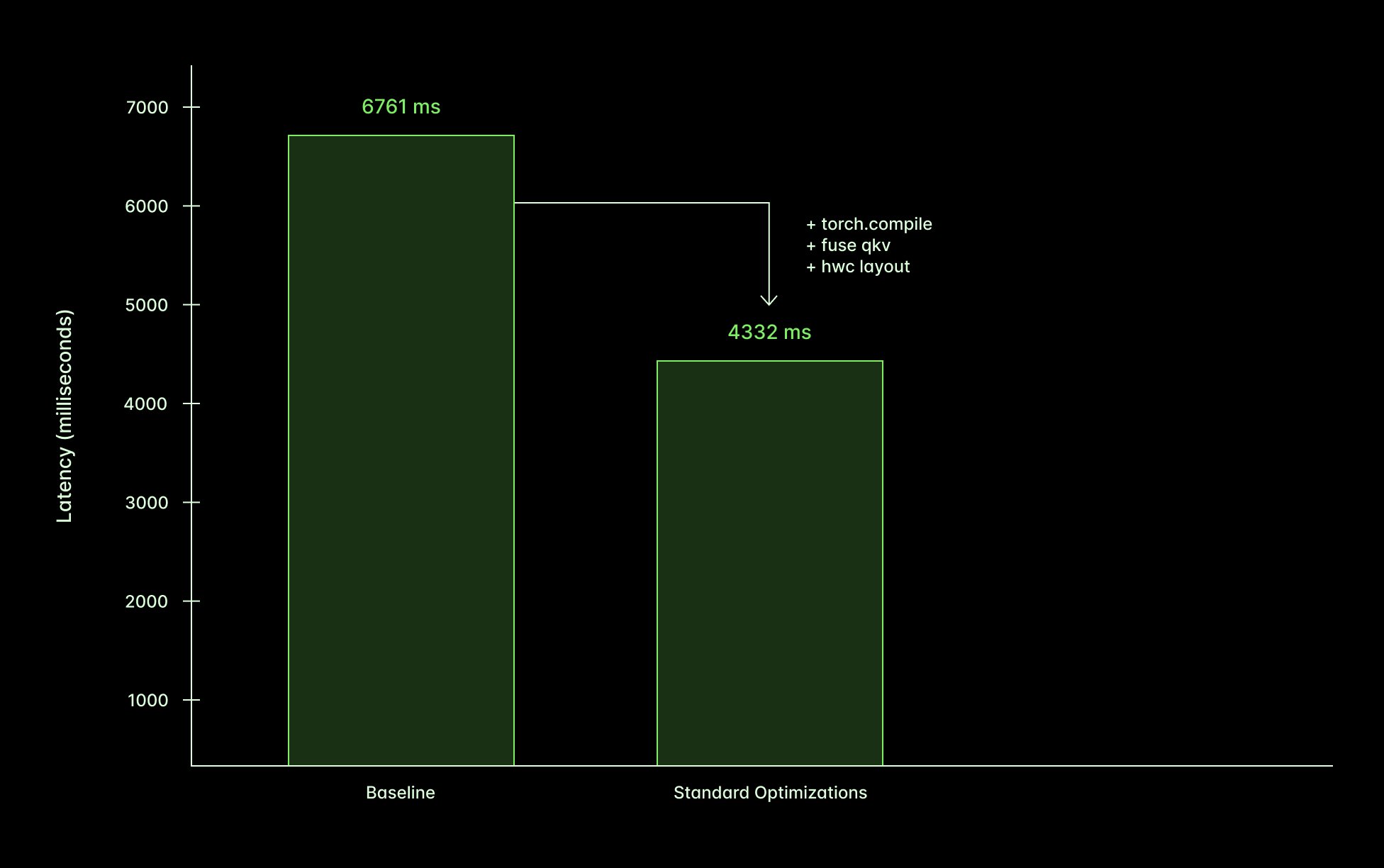
Applying the “standard” optimizations (running the Torch compiler, switching the data layout, and fusing the QKV calculation) got us halfway to the target.

Then we applied a fun, approximate activation caching technique, First Block Caching, and cut the latency in half again.

Implement the baseline

Before beginning to improve performance, you need to first measure the current performance cleanly.

We start with the standard Hugging Face diffusers library and create our FluxPipeline in 16bit precision.

self.pipe = FluxPipeline.from_pretrained(
    "black-forest-labs/FLUX.1-dev",
    torch_dtype=torch.bfloat16,
    use_safetensors=True,
)

Averaging across a variety of inputs, we find that we can generate a 1024x1024 image in ~6.75 seconds.

Apply standard optimizations for a 1.5x speedup

We started by applying a bunch of “standard” optimizations — using Torch’s optimizing compiler; fusing the query, key, and value computations in the Transformer attention; and using the “channels last” memory layout. These are nearly always a good idea.

Optimize the compute graph with the Torch compiler

What is a PyTorch program really? By default, PyTorch constructs a compute graph of tensor operations dynamically in Python and runs it eagerly. This “virtual compute graph” is executed on the host/CPU and triggers execution of a “real compute graph” on the device/GPU. If you’re curious how this works, we recommend generating some PyTorch traces and examining them.

Graph representations of programs are really nice for program transformations. Back in the BC era (Before ChatGPT), most people used PyTorch to train their own neural networks, and the key program transformation was running the program backwards to figure out how to make it less wrong, aka “learning representations by back-propagating errors”.

Now that, like neural networks themselves, PyTorch is used more for inference, the key program transformation has changed to compilation. Compilation replaces the compute graph with an equivalent but faster one. If you’re familiar with database query compilers, think of logical-logical optimization transformations like predicate pushdown.

As with any respectable modern compiler, the Torch compiler operates as a series of lowerings into increasingly concrete intermediate representations. TorchDynamo hooks the CPython frame interpreter, traces Python bytecode, and carves out stretches of Tensor operations into lowered “FX” graphs. A backend compiler like TorchInductor then takes these graphs and lowers them to a further optimized representation, like a Triton kernel.

We separately compile the model’s two large subcomponents (the Transformer and the Variational Autoencoder). Our configuration settings appear in the code snippet below. We got many of them from this excellent guide on Hugging Face and did some light validation before adjusting other parameters.

The most notable choice is to use max-autotune, which incurs tens of minutes of compile-time cost but ensures optimal run-time performance. See the final section for details on how we cut that back down to minutes without losing Modal’s transparent auto-scaling.

class Flux:
    ...

    @modal.enter()
    def setup(self):
        self.pipe = FluxPipeline.from_pretrained(
            "black-forest-labs/FLUX.1-dev",
            torch_dtype=torch.bfloat16,
            use_safetensors=True,
        )
        # torch.compile configuration
        config = torch._inductor.config
        config.conv_1x1_as_mm = True
        config.coordinate_descent_check_all_directions = True
        config.coordinate_descent_tuning = True
        config.disable_progress = False
        config.epilogue_fusion = False
        config.shape_padding = True

        # Mark layers for compilation with dynamic shapes enabled.
        self.pipe.transformer = torch.compile(
            self.pipe.transformer, mode="max-autotune-no-cudagraphs", dynamic=True
        )

        self.pipe.vae.decode = torch.compile(
            self.pipe.vae.decode, mode="max-autotune-no-cudagraphs", dynamic=True
        )
        # Trigger torch compile
        self.pipe("dummy prompt", height=1024, width=1024, num_images_per_prompt=1)
        ...

Expose more parallelism to the GPU with fused QKV

FLUX includes a big Transformer model. The Transformer architecture’s signature component is the attention block, which transmits information between text and image and through internal circuits. They are usually written in terms of three separate matrix multiplications between the block’s input matrix X and its weight matrices W_q, W_k, and W_v.

If we concatenate the three weight matrices, we can perform the attention calculation as one large matrix multiplication: (QKV = X @ W_qkv). This exposes more of the parallelism in the operation to the lowered representations. In particular, X is the same matrix for the entire multiplication, not three variable references that we totally promise the Torch compiler must verify are to the exact same data.

class Flux:
    ...
    @modal.enter()
    def setup(self):
        ...
        self.pipe.transformer.fuse_qkv_projections()
        self.pipe.vae.fuse_qkv_projections()
        ...

Improve data locality with channels-last memory layout

The last standard optimization we do is a common recommendation to improve data locality.

Tensors are spicy multi-dimensional arrays. Tensors representing images (or feature maps over images) have three dimensions: channel (color), height (y position) and width (x position). This three-dimensional array needs to be mapped onto linear computer memory.

By default, PyTorch orders image Tensors in memory by channel first, then by height, then by width (CHW or “Channels First”). Sequential accesses therefore read spatially nearby values from a single channel/color.

Let’s walk through an example. This image

// a 2x4 image with three channels of one byte each
┌────────┬────────┬────────┬────────┐
│ #888888│ #999999│ #AAAAAA│ #BBBBBB│
├────────┼────────┼────────┼────────┤
│ #CCCCCC│ #DDDDDD│ #EEEEEE│ #FFFFFF│
└────────┴────────┴────────┴────────┘

is represented in memory in CHW format as

// channels first
0x00 : 88 99 AA BB  CC DD EE FF   ← 🟥 red values
0x0F : 88 99 AA BB  CC DD EE FF   ← 🟩 green values
0x17 : 88 99 AA BB  CC DD EE FF   ← 🟦 blue values

But many operations in neural networks, like convolutions, are global across channels and local in space. That means we usually want to access all channels at a particular set of positions, and so we want channels to be last.

// channels last
0x00 : 88 88 88   🟥 🟩 🟦
0x03 : 99 99 99   🟥 🟩 🟦
0x06 : AA AA AA   🟥 🟩 🟦
0x09 : BB BB BB   🟥 🟩 🟦
0x0C : CC CC CC   🟥 🟩 🟦
0x0F : DD DD DD   🟥 🟩 🟦
0x12 : EE EE EE   🟥 🟩 🟦
0x15 : FF FF FF   🟥 🟩 🟦

You can convert PyTorch models into this format with the memory_format argument.

class Flux:
    ...
    @modal.enter()
    def setup(self):
        ...
        self.pipe.transformer.to(memory_format=torch.channels_last)
        self.pipe.vae.to(memory_format=torch.channels_last)
        ...

Putting it all together, we get a 1.5x speedup

The performance improvement of these optimizations in aggregate is about 1.5x, driven mostly by the Torch compiler.

This speedup is definitely respectable, as evidenced by the animation below, which shows the evolution of the image across denoising steps, rendered at the same rate those steps execute for the two methods.

Apply vibes-based approximate caching for another 2x speedup

Applying the “standard” optimizations above is pretty straightforward and ends up being an appealing point on the engineering effort/performance curve. But we needed to go further on performance, so we needed to go deeper.

Diffusion models generate images iteratively, turning noise into art, one step at a time. That’s the process we’re showing in these animations. If you look closely you can see that during some steps, the image doesn’t change much at all.

As it turns out, if you’re willing to tolerate some slight changes in the results, you can skip those steps entirely!

This is an important difference between neural networks and other programs. With neural networks, you can often remove chunks or skip steps, and the program still runs, and does “almost” the same thing. More like an analog computer than a digital one!

We used the “first block caching” technique and implementation from the ParaAttention repo, itself based on the approach from the TEACache paper. The basic idea is to start running the model for a timestep. If, partway through the model’s forward pass (after the “first block”), it looks like there won’t be a large change, you skip the step.

class Flux:
    ...
    @modal.enter()
    def setup(self):
        ...
        from para_attn.first_block_cache.diffusers_adapters import apply_cache_on_pipe
        apply_cache_on_pipe(
            self.pipe,
            residual_diff_threshold=0.12,
            # quality degraded too much at higher thresholds
        )

The definition of “large” is a tunable parameter, where higher values lead to larger changes in model behavior but faster execution. This allows for a smoother tradeoff between performance improvement and quality degradation than other techniques that do the same, like quantization.

We got a 2x speedup with a threshold of 0.12 and images looked better than with the default of 0.08, so we stuck with it.

Cut cold start latency by 30x with caches and snapshots

As we optimized inference, we took an enormous hit on boot time — from seconds to tens of minutes.

Boot time matters for cost and speed as well. If boots are fast, you can run only as many replicas as you need to satisfy current demand and still hit your latency objectives.

This is something we think is very critical, and we spend a lot of time optimizing this at Modal! You can read more about why we think this is so important for generative applications in our GPU utilization explainer and our case study with Suno.

The primary culprit is the Torch compiler, and specifically max-autotune, which profiles multiple implementations at compile time to find the fastest one.

This is a classic use case for a cache — compute-intensive work that produces serializable artifacts. Torch Compile offers both piece-wise caching of smaller artifacts, like compiled Triton kernels, and a “megacache” that stores entire cached compute graphs. We used both, but the megacache didn’t offer a large speedup. It didn’t hurt either, and it’s a new feature we expect to improve over time, so we left it in. You can find the details here.

We also shave off a few seconds using Modal’s memory snapshots feature, which lets us turn the many file reads and code execution in import torch and from_pretrained into a single file read (for every invocation after the first). Check out this blog post for a deep dive.

image = image.env(
	{
        "TORCHINDUCTOR_FX_GRAPH_CACHE": "1",
        "CUDA_CACHE_PATH": "/cache/.nv_cache",
        "TORCHINDUCTOR_CACHE_DIR": "/cache/.inductor_cache",
        "TRITON_CACHE_DIR": "/cache/.triton_cache",
	}
)

CACHE_VOLUME = modal.Volume.from_name("cache_volume", create_if_missing=True)

@app.cls(
    enable_memory_snapshot=True,
    volumes={"/cache": CACHE_VOLUME}
    ...
)
class Flux:
    @modal.enter(snap=True)
    def load(self):
        self.pipe = FluxPipeline.from_pretrained(
            "black-forest-labs/FLUX.1-dev",
            torch_dtype=torch.bfloat16,
            use_safetensors=True,
        ).to("cpu")

    @modal.enter(snap=False)
    def setup(self):
        self.pipe.to("cuda")
        ... # rest of setup

Serve AI models at scale with Modal

Together, these optimizations cut FLUX.1-dev serving latency to match the performance of proprietary serving APIs. On Modal, that means you can match or beat providers on price too.

We didn’t talk too much about all the other problems that come up when building and serving a generative API — interactive development, handling bursty loads, and training/evaluating the next iteration of the service. If that’s interesting to you, check out the Modal serverless platform, trusted to run generative inference at the scale of thousands of GPUs and tens of thousands of CPUs by customers from Suno to Substack to soccer teams.