






Software is eating the world, and agents are eating software engineering. It is imperative that software engineers develop an understanding not just of the agent software that is now their most important tool but also of how the intelligent core of agent software works, through inference by large generative models of language — if not out of the engineer’s need to understand and control their tools, then at least because inference is poised to consume more computing power and produce more benefit than all other uses of computers.
The central fact about inference services for coding agents is that they must operate at extremely high relative and absolute performance.
By relative performance, we mean large fractions of the peak rate or “speed of light” of the hardware that it uses. By absolute performance, we mean that the scale of that peak rate and the amount of work done per request is large. Contemporary matrix math accelerators like Tensor Cores operate at the petaFLOP per second scale. Large generative sequence models with sufficient intelligence to automate software development have trillions of floating point parameters, and each of them must be accessed many times per second, even when serving just a single request.
Due to these requirements, economically viable coding agent inference services are currently only feasible by operating at a scale sufficient to amortize hardware and engineering costs — roughly, at the scale of trillions of input and output tokens.
We’ve done this, and we’d like to share how.
At Modal, we operate a number of such inference services for coding agents at this scale and work with a number of customers who do the same. You can use our services indirectly via inference routing platforms like OpenRouter or Vercel AI Gateway or directly through our Shared Endpoints.
In this blog post, we will walk through how we optimized inference performance when serving inferences from Moonshot AI’s Kimi K2.6 model to power coding agents. Though this model is “old” by this field’s standards (literally hundreds of days old!), the fundamentals of sequence modeling, hardware, and scaling change slowly enough that the core story and many of the details match what we have done for more recent models that have superseded K2.6 in intelligence and cost-performance, like Kimi K3.
Our optimizations allowed us to scale per-replica performance of inference replicas by 2.8x per user and 5.6x across users on the replica:
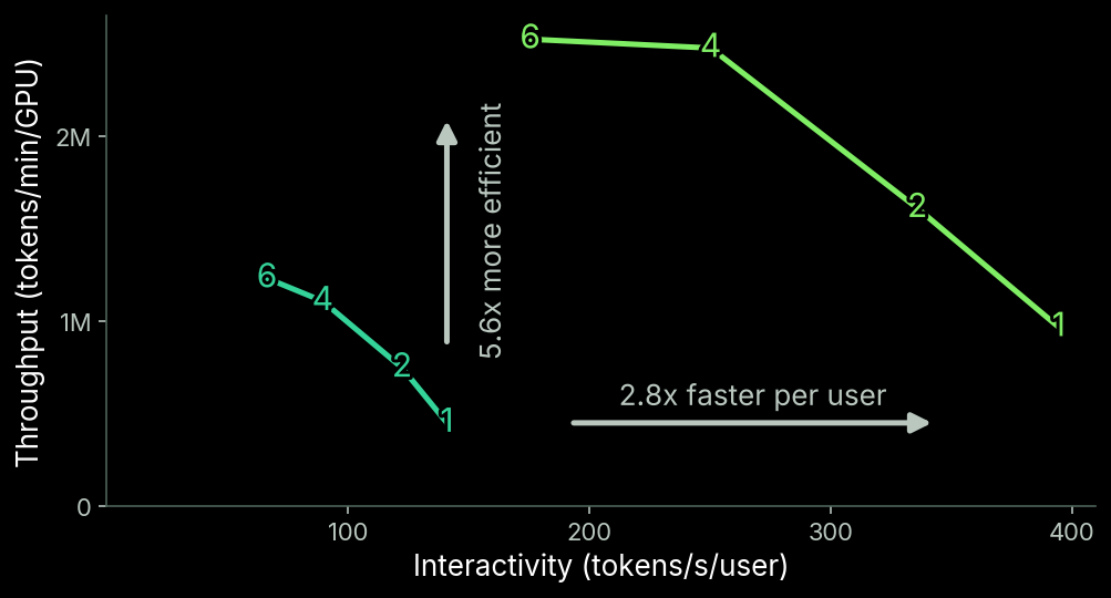
This chart relates the individual user’s experience (decode tokens per second per user, aka interactivity) on the x-axis with the cost-performance of the overall system on the y-axis (total tokens per minute per GPU, aka token throughput), with the number of concurrent users indicated at each point.
More intuitively, that’s the difference between a ruinously expensive service with the UX on the right below and a price-competitive service with the UX on the left:
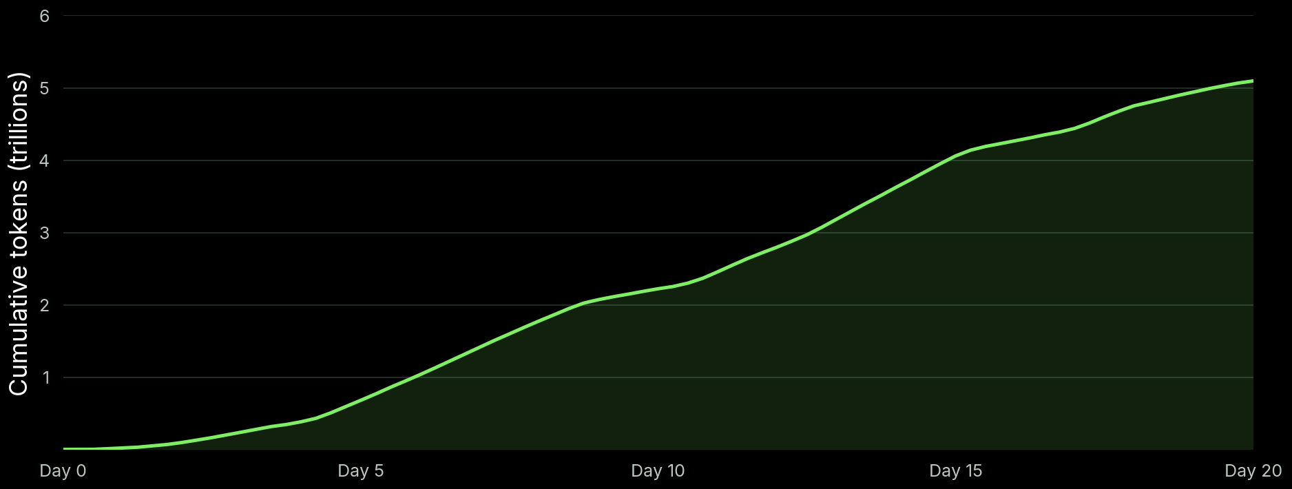
We then scaled those single-container replicas into deployments and services. One particular service processed hundreds of billions of tokens a day and trillions in aggregate:
Below, we aim to make this performance engineering legible to a general software engineering audience. By sharing how we, and our customers, are able to operate these services, we hope it enables you to do the same — perhaps by deploying a Dedicated Endpoint on Modal.
First, understand the workload.
We break this down into two sections: understanding the sequence model that infers the response to each request and understanding workload structure across requests.
State-of-the-art coding agents are supported by trillion-parameter neural sequence models that process input in parallel and infer output sequentially.
Contemporary coding agents are powered by probabilistic generative models of unicode sequences pre-trained mainly via unsupervised masked sequence prediction and post-trained mainly by reinforcement of output software correctness. Like the parser of a compiler, they operate not on raw strings but on tokenized sequences, so we call their inputs and outputs tokens. Because we are, in the end, guessing what output tokens should be, this is called inference. If you prefer deduction, stick to databases and operating systems.
The underlying sequence models these days are hybrid-attention, mixture-of-experts Transformer neural networks. These networks apply computations both per token in the sequence and across tokens in the sequence.
Attention has evolved into a generic term for cross-token computation. Mixture-of-experts refers to the dynamically routed block-sparse matrix multiplication that applies the majority of the per-token computation. These computations iteratively update the network’s internal, or latent, representation.
For insight into what’s going on inside these sequence models, see Anthropic’s “A Mathematical Framework for Transformer Circuits” (2021, but still undefeated).
A single forward pass through such a neural network produces both substantial internal state and a probability distribution over the next token(s) in the sequence for each sequence position. Because we predict (”regress”) based on our own outputs (”auto”), this is autoregressive sequence modeling.
To respond to a client request, we generally chain multiple forward passes together like this:
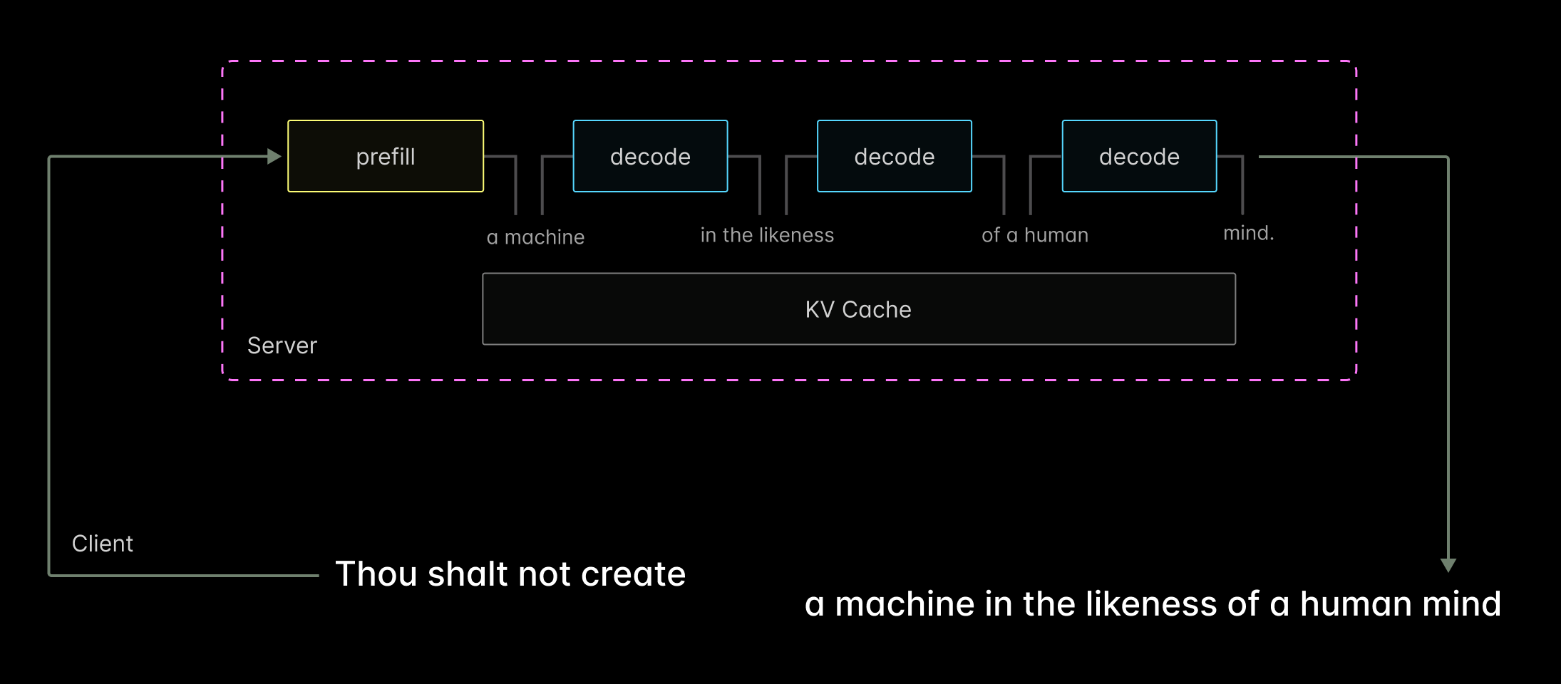
Forward passes are expensive, so we want to amortize this work as much as possible. Much of the work in per-token computation amortizes by batching several sequences together. Much of the work in cross-token computation amortizes by caching the internal state. For historical reasons, this is called the key-value cache (KV cache or just KV), even though contemporary models like Kimi don’t have distinct keys and values. You can read more about the “napkin math” here in Kipply’s excellent “Transformer Inference Arithmetic” blogpost (2022, but still undefeated).
When a forward pass processes a request’s input tokens, we call it a prefill, because it is “prefilling” the KV cache. When a forward pass produces a response’s output tokens, we call it a decode, because we are “decoding” the model’s “encoding” of past state into predicted future. What about forward passes that do both? Yeah, we don’t like the terminology either.
Prefill performance is mostly tracked by the latency to complete all prefills for a request, aka time-to-first-token (TTFT). Decode performance is mostly measured by the rate at which output tokens are produced after that, aka output tokens per second (TPS). Both can be measured client-side or server-side, causing no end of confusion.
The particular sequence model covered in this post is Kimi K2.6 by Moonshot AI. This model parametrizes its matrix multiplications with approximately one trillion numbers (weights in its matrices), the majority of which are stored as four bit integers (INT4).
We serve the model, however, with four bit floating point numbers (FP4). Four bits only gives you sixteen distinct values, so you further need a micro-scaling format to scale individual blocks within tensors independently. We chose the NVFP4 micro-scaling format, which has native hardware support at the petaFLOP/s scale in the Tensor Cores of Blackwell Streaming Multiprocessor Architecture GPUs like the B200 and B300. Because we operate a dynamic GPU fleet in a time of constrained compute supply, we prepare our deployment to run on both B200 and B300 GPUs. Results below are all for B200 GPUs; B300s are substantively similar but operate at higher request concurrency because they have more high-bandwidth memory (HBM) available for caching.
We chose the SGLang inference engine as our base. We found several opportunities to improve performance by patching the engine. As contributors to the SGLang project, we upstreamed these patches, described and linked in the post below.
To optimize UX and cost-performance, you must understand the structure of these sequences across requests.
When you serve such models on coding agent traffic naïvely, you get bad results.
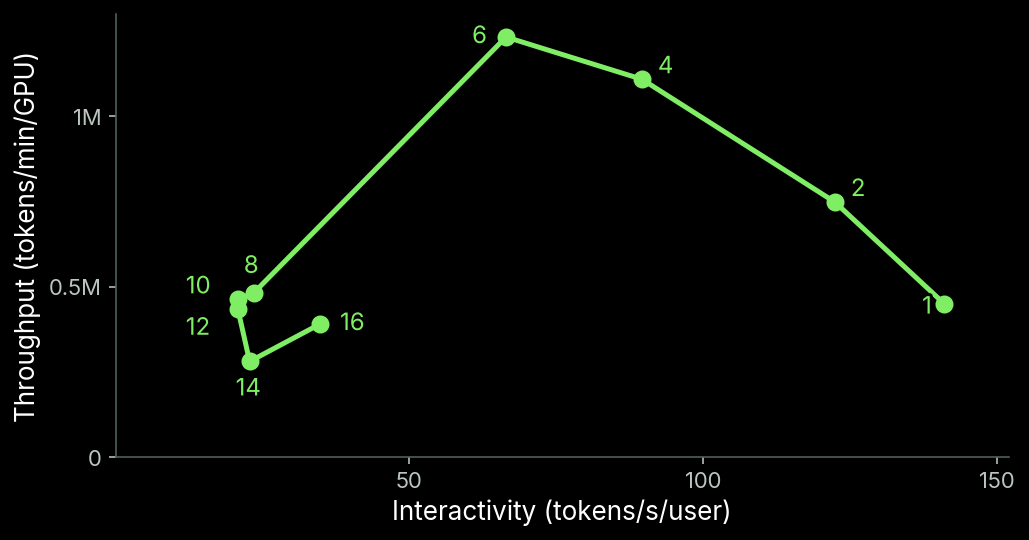
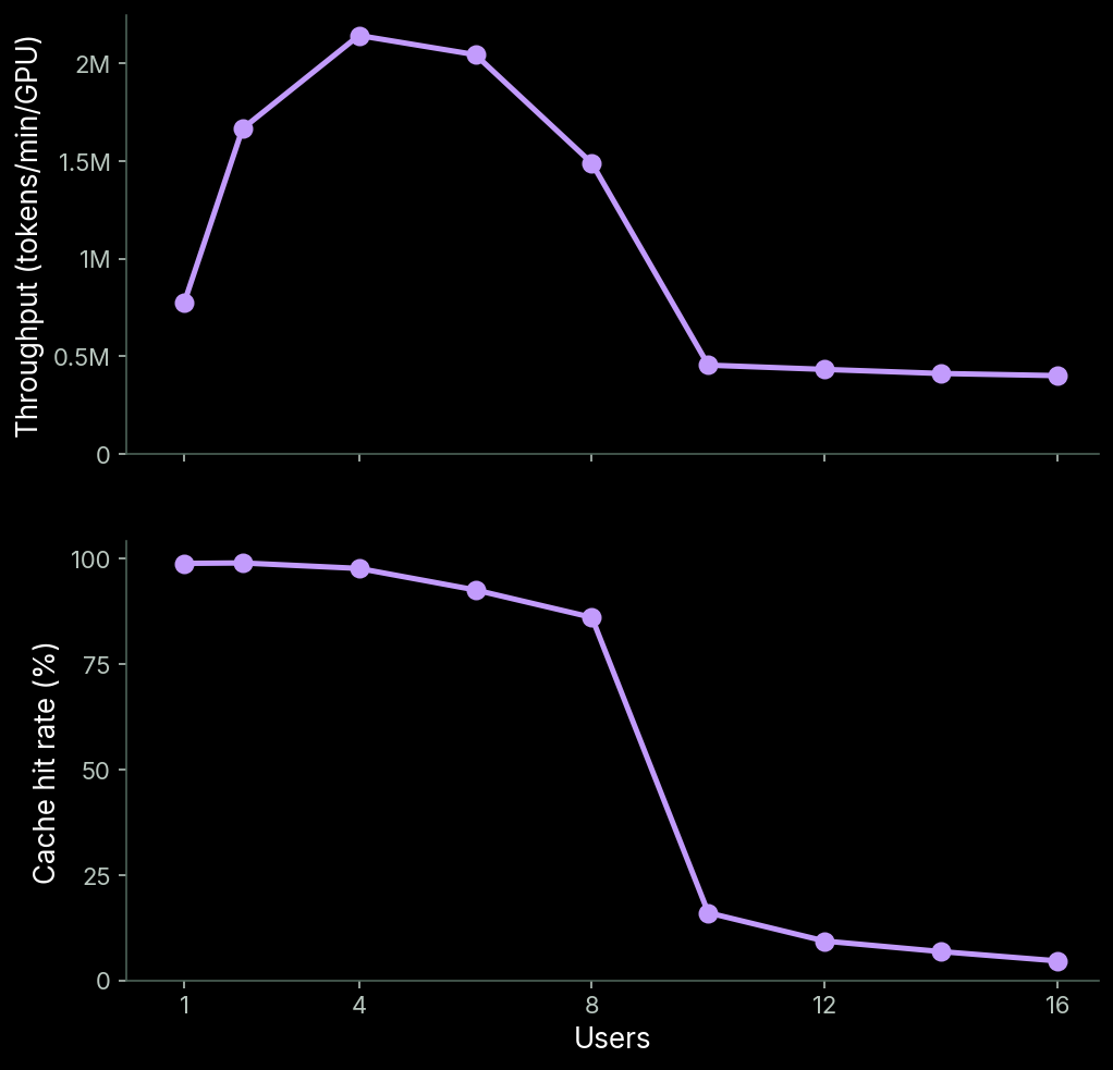
This chart indicates that throughput and interactivity rapidly collapse above 6 concurrent users. Furthermore, even before that peak, the interactivity is below user expectations and the system is below acceptable efficiency.
So from here, you need to increase interactivity and throughput to deliver better outcomes to users while decreasing your own costs. To do that, you need to understand the sequences in this workload deeper than just “tokens in and tokens out”.
Individual requests for output tokens are created in “sessions”: the user, the generative model, and the tool calls chain together iteratively to construct a tower of input sequences, accumulating context — and value — over time. The iterative process of meaning construction, information discovery, and sense-making strikes us as fundamental to the nature of sequence modeling and sequential action, so we expect this pattern to far outlast “coding agents”.
Concretely, a single session looks something like this:
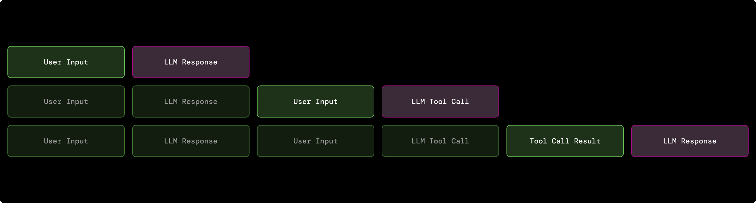
That is, the input sequence (green) for each turn T is the entire session history up to T (darker green), plus something new (lighter green). This has two key consequences.
First, it means requests inherently have long input sequences relative to their output sequences (pink, above) — there are T-1 past output sequences in the input to turn T, and T is in the dozens. For the core workload we used in optimization and served in production, this ratio was 200:1; requests contain roughly 100k input tokens and produce roughly 500 output tokens. That means the majority of processed tokens will be input tokens (just check the token usage numbers in your coding agent software).
Second, it means the input sequences have high overlap with previously processed input sequences — the ones from turns 1 to T-1. That means that on the way to serving turn T, the tokens in turn 1 are processed T times. This makes caching absolutely critical — we can avoid linearly-scaling recomputation to save effort, but we introduce linearly-scaling state that must be managed and has its own performance characteristics. Navigating this tradeoff is the core engineering problem we’ll tackle in this post.
With this picture of the workload in mind, we turn to optimization.
Then, optimize a single replica.
To optimize performance, build a working system, identify the bottleneck, then lift it. Repeat as needed until you’ve won.
Though our ultimate goal was to optimize an entire service, we decomposed that problem into two simpler problems: optimize a single replica first, then scale from one to many replicas.
We further split the problem of single replica performance into two sub-problems: first maximize interactivity, then maximize throughput without losing interactivity.
Interactivity primarily impacts request latency. Request latency and throughput interact through concurrency, the number of in-flight requests, by a rearrangement of Little’s Law:

Our key bottlenecks for latency, concurrency, and throughput started in the GPU HBM.
Our key bottleneck on latency was HBM bandwidth during decode. We lifted it by parallelizing matrix multiplication across GPUs (tensor parallelism, TP) and by applying custom DFlash speculative decoding — doing more computation per memory load, even when that computation may not be needed.
That created a bottleneck on concurrency through HBM capacity: how much work can we keep in a cache that loads faster than we could just recompute results. We lifted it by clearing up intermediates in HBM, quantizing intermediates to lower floating point precision, and extending the cache hierarchy to CPU RAM with HiCache. We used the cache hit rate (CHR) as a targeted metric of improvements to caching. CHRs between one and two 9s are very much feasible for most coding agent workloads.
We started by maximizing interactivity.
Increasing interactivity increases the system performance as observed by individual users. We chose to work on this first. We made that choice for several reasons.
First and simplest, we found that coding agent users enjoy and will pay more for tokens that come to them faster, so high interactivity was key to building the service that our and our customers’ users wanted.
Second, interactivity is particularly amenable to improvement by speculative decoding. Because it is a simple, learning-based technique, its performance benefits scale with compute and data: machine learning’s famous “bitter lesson”, returning in performance engineering for ML systems. And we know how to scale training.
This choice to interactivity-maxx had two additional benefits, one operational and the other for throughput, which were especially salient because we operate a dynamic, autoscaling fleet of thousands of GPUs.
Maximum interactivity replicas are smaller and therefore easier to serve.
Using multiple processors together requires an interconnection network (interconnect) for communication. The lowest latency, highest bandwidth interconnect for Nvidia GPUs is NVLink. NVLink operates across a group of processors in a “domain” of some size.
A single host operating system can support an NVLink domain of up to 8 GPUs. The largest NVLink domains that are generally available comprise 72 accelerators (in a multi-node IMEX domain). Using more accelerators would require a slower interconnect (IB/RoCE or, worse, standard Ethernet). That means that for maximum interactivity we should not expect to use more than 72 accelerators per replica — the communication overhead will almost surely dominate any per-request latency wins.
But that doesn’t mean we must use 72 accelerators.
Consider these results from SemiAnalysis’s InferenceX benchmarks for this same NVFP4 Kimi K2.6 model, which show throughput per GPU as a function of interactivity, annotated with GPU count, for a variety of deployments:
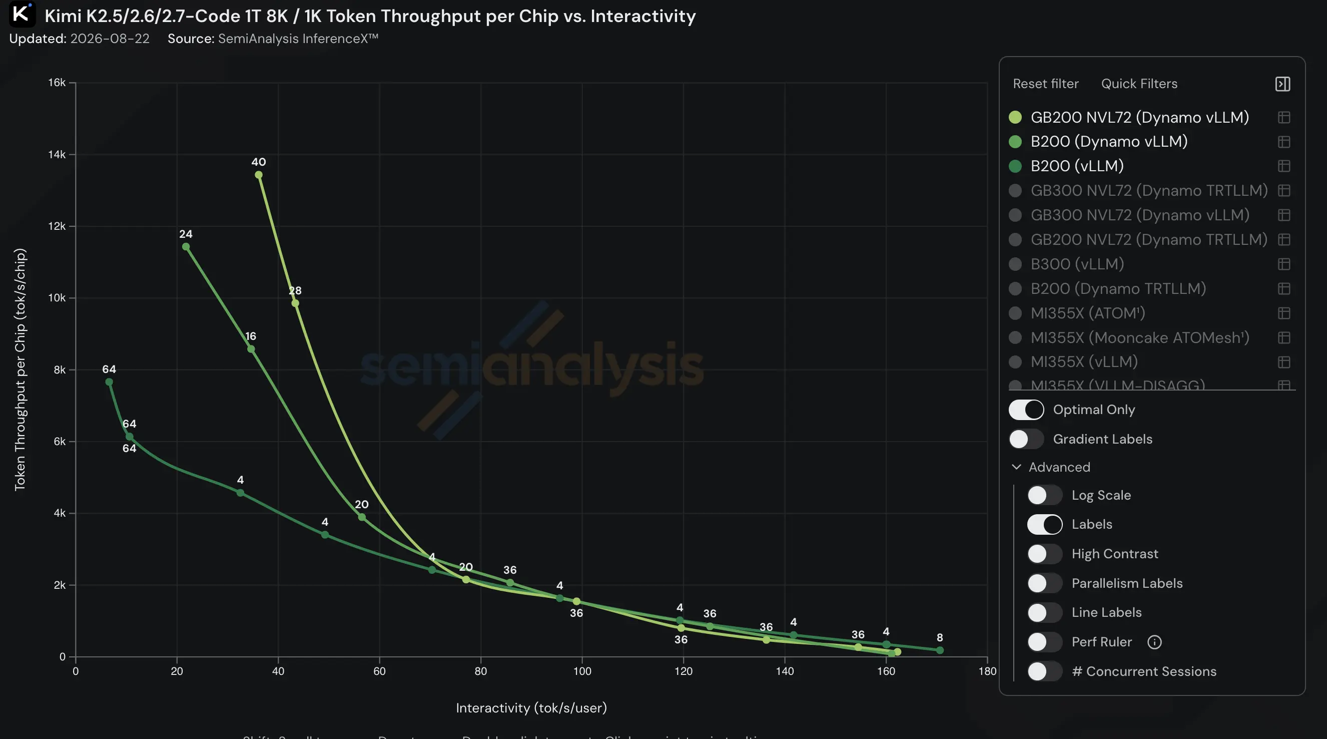
The highest interactivity is achieved by a deployment with just eight GPUs per replica. Furthermore, that interactivity is achieved with comparable throughput per GPU, which means that by choosing a smaller domain, we are not obviously forgoing peak throughput cost-performance (subject to our interactivity constraint).
To keep the chart legible, we selected only a small subset of deployments most similar to ours, but the pattern holds across more accelerator types and across more models in the InferenceX benchmarks (explore them here). Generally, you can achieve the highest interactivity at comparable per-GPU throughput with only four or eight GPUs. You can then achieve the same aggregate throughput by scaling smaller replicas. The core Modal serverless platform makes this scaling performant and reliable.
This is a huge operational win. Smaller, simpler units make for easier scaling. Eight GPUs can be driven by a single host OS kernel. An NVL72 domain, on the other hand, is comprised of nine such subsystems sharing an address space (yes, you should be shuddering). Availability is constrained and contracts are long and inflexible.
Eight-GPU Blackwell systems, on the other hand, are standard enough to be available via on-demand and spot markets, which makes it much more cost-effective to handle variable load. Replicas with one, two, or four GPUs can furthermore be packed inside of a single physical eight-GPU machine — which already has all the resources required to start another replica (model weights, JIT artifacts).
Of course, as and if the compute supply and user demands change, we will happily revisit this choice.
Increasing interactivity indirectly increases throughput.
By reducing the latency of individual requests, we indirectly improve throughput by freeing up resources for new requests.
Agentic coding workloads are approximately “closed-loop” per session. Sessions are almost always chains — of user-written tokens, of tool call responses, and of model outputs. The next request in the session, therefore, almost always arrives some time after the previous response has finished generating. The session’s next request is therefore latent for some time, outside the inference system — for tool calls, 10s of ms to seconds with a tail of minutes; for user responses, seconds to minutes, with a tail of hours or more.
During that time, other requests can be processed on the same node. When you have sufficient load for the active capacity, there are always requests ready for a node to process. When you have sufficient capacity for the active load, there are always nodes to map requests onto. Both of these are guaranteed by our fast autoscaling system. We’ll talk more about request routing in the section on scaling to multiple replicas.
Use custom speculative decoding to do more work each time you hit the bottleneck on interactivity.
Interactivity measures output tokens per second per user. Naïvely, autoregressive sequence models like Transformers produce these tokens sequentially. Amdahl’s heartbreaking Law strikes again.
Each time a token is produced, gigabytes or more of model weights and KV cache must be loaded from GPU HBM to Streaming Multiprocessor L1 caches, which generally takes longer than actually computing the KV state and output for a single next token. This creates a bottleneck on that memory bandwidth. Parallelism helps create more bandwidth, but this is more useful for per-token calculations than for cross-token calculations, which arise as a bottleneck for long sequences, as observed in coding agent workloads.
So we instead elevated that bottleneck by applying speculative decoding.
Fundamentally, speculative decoding makes the same trade that speculative execution in processors makes: when you have spare operational bandwidth due to serial dependencies between operations, you can use that bandwidth to run operations that may not end up being used. Effective operational throughput increases if you can guess operations that will be used with high probability, and the name of the game is increasing that probability with the least work possible.
For autoregressive sequence model inference, the “trick” to run more operations per iteration is to guess what the next several tokens will be using another, faster language model (the “speculator” or “draft”), and then validate the guesses in parallel with the served model (the “target” or “verifier”).
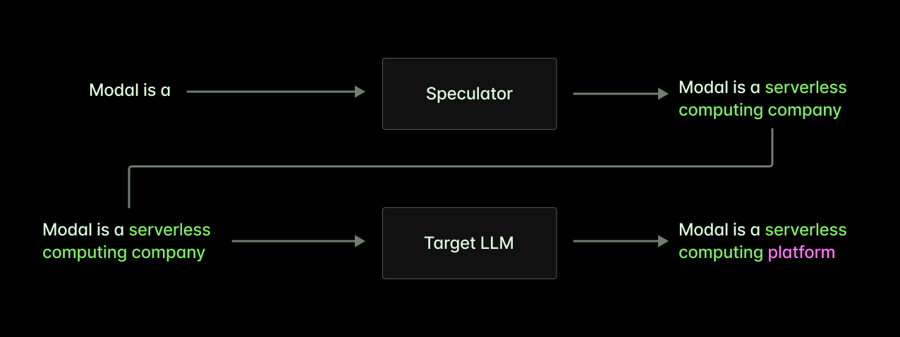
As with speculative execution, this acceleration happens without changing program behavior, i.e. the probability distribution of the target sequence model.
As we describe in our blog post releasing speculators for the Qwen 3.5 and 3.6 model family, the gains from speculative decoding are large — integral factors, not a few tens of percent.
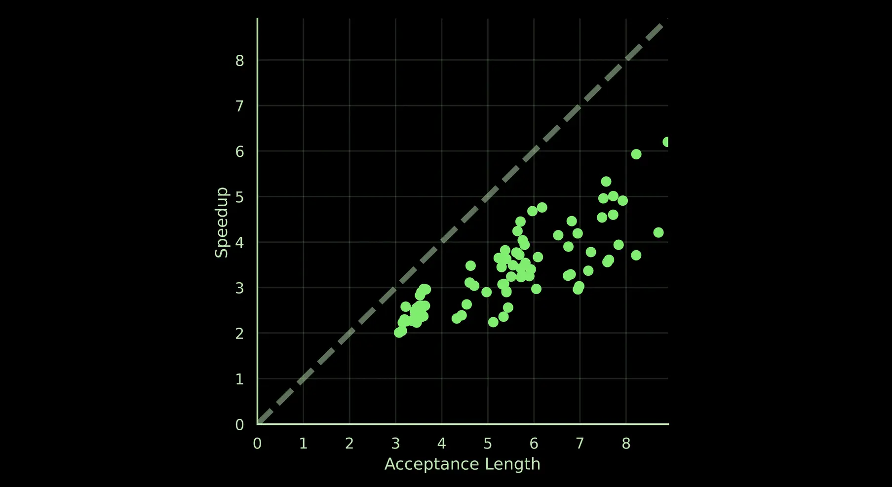
Counterintuitively, it is fairly easy to produce a speculator that predicts four, eight, or even more of the next tokens in the output, on average, especially for coding agent workloads. Roughly, there are two reasons this is the case: the target model sets speculators up for success and the majority of tokens do not use the full intelligence of the target model.
Speculators can re-use the work of the target model.
First, the target language model has already produced extremely useful representations of the sequence during its forward passes — starting from the static embedding of each token, each layer of the model progressively enriches this representation, up until the final “language modeling head” layer turns that representation into a distribution over next tokens. Even better, these representations are already stored in KV cache. State-of-the-art speculator architectures like DFlash (and derivatives like DSpark) re-use this state as their inputs, so they can be orders of magnitude smaller (and faster) than the target: standing on the shoulders of giants, pointing to where they might go next.
Token sequences are repetitive and low in information density.
Consider the following sample coding agent output:
You're absolutely right! I should have read that file before I
"straight yeeted it to prod". Checking now.

Tool call: Read src/config.py L42-L96
Anyone who has used recent models can give you a good guess for what comes after You’re absolutely (it's never wrong). And the quotation is from previous user input, so once the quote opens, the next tokens become highly predictable.
Looking a layer deeper, consider what this sequence looks like once it has been formatted with the special control tokens in the model’s “chat template”:
<|im_assistant|>
	You're absolutely right! I should have read that file before I "straight yeeted it to prod". Checking now.
	<|tool_calls_section_begin|>
		<|tool_call_begin|>functions.Read:0
			<|tool_call_argument_begin|>
				{"path":"src/config.py","line_start":42,"line_end":96}
			<|tool_call_end|>
		<|tool_calls_section_end|>
	<|im_end|>
This sequence has substantial structure that does not require high intelligence to produce. Of course, the details within that structure still matter for correctness, so the target model’s capabilities are still important!
Most of the capacity of the target model, then, is likely going to enrichment of the representations of these tokens for use in predicting tokens many steps ahead. If you already know what the next several tokens are, you can compute their representations in parallel.
This is not a quirk or a hack: providing dual parallel and sequential forward passes is a fundamental feature of modern sequence models relative to traditional recurrent neural networks. It is present in both “classic” Transformers and linear/hybrid attention models, so we can expect it to persist.
For this and other reasons, we have invested heavily in speculative decoding, and we suggest you do the same.
Custom speculators can dramatically increase acceptance lengths.
The fastest speculators are trained not just to predict the general behavior of the target model but to predict its behavior on specific datasets. Because they are small, their modeling capacity is limited, and you want to use that capacity only for what will actually occur in production. For the ML ‘heads: the loss for a speculator is Kullback-Leibler divergence from the target model, which encourages mode-seeking, rather than mode-covering.
But as with neural networks in general, our experiments have indicated that it’s better to start from a strong foundation and then adapt the speculator to the specific task — aka fine-tuning. So we first trained a DFlash speculator for Kimi K2.6 on a generic data mixture and then fine-tuned it on coding traces that were output by the target model. The draft model can then be continually trained on the target model’s outputs when serving production traffic.
We ran into one issue when operating on live traffic: mapping tokens to a string and then re-tokenizing is not an identity map, because tokenization is fundamentally a cursed hack. But typical logging, e.g. of HTTP requests, operates on strings, not tokens. We therefore patched SGLang to emit raw token ids through sglext and contributed the work upstream.
Fine-tuning gave us an increase in accept length from 5.00 to 5.84 tokens per step on representative traces, for an incremental speedup of 20%.
Tensor parallel was the best parallelism strategy for maximum interactivity.
Adding more engineers to a slow task makes it take longer, but computers have no such weakness — if you parallelize work and shard data correctly.
The primary parallelism strategies for sequence model inference split work:
- within a single request, across model forward passes (prefill-decode disaggregation),
- within a model forward pass, across layers (pipeline parallelism),
- within a batch of requests, across sequences (data parallelism),
- within a sequence, across tokens (context parallelism),
- within a model layer, across matrix multiplications (expert parallelism), and
- within a matrix multiplication, across rows/columns (tensor parallelism).
Of these choices, only context parallelism, expert parallelism, and tensor parallelism split work within a single request and so directly improve interactivity. Tensor parallelism (TP) is the lowest level of parallelization — besides the parallelism within kernel execution, which is legion but out of scope (we’ve shared some of our work on that elsewhere). That means TP optimizations compose better with other strategies and therefore make a good first target.
In more detail: tensor parallelism takes an input to a matrix multiplication and splits the output processing work across parallel workers, which can therefore shard the matrix data needed for that processing, aka the model weights. For more, see the Megatron paper (2019, but still undefeated).
Despite this first-principles argument, we still investigated multiple other parallelism strategies, because 1) interactivity can be indirectly affected by optimizations elsewhere and 2) you never know what you don’t know. However, we found that Tensor Parallelism Is All You Need™ to interactivity-maxx. For instance, we found that data-parallel attention allowed us to achieve higher concurrency by sharding KV cache, but latency was worse. In fact, it was so much worse that it caused overall throughput per GPU to drop, even though concurrency increased.
Along with choosing a parallelism strategy, you also need to choose the number of parallel workers. For the Kimi K2.6 model running on B200 GPUs on sequences that may have hundreds of thousands of tokens, the feasible configurations are with four GPUs (TP4) and with eight (TP8).
Some quick napkin math there: a B200 has 180 GB of HBM, and Kimi K2.6 has 595 GB of weights (over a trillion, one nybble per weight). Spilling weights to CPU RAM or disk would wreck latency, so TP1 and TP2 are both infeasible. With four or eight GPUs to shard weights over, we have about 125 or 845 GB for KV. Each KV entry has 576 elements, stored in two-byte BF16 format, and there are 61 layers, each with their own KV entry per token, and so a single token consumes ~72 KB = 576×2×61 bytes. That gives you space for about half a million tokens of KV in TP4, or about three million in TP8 — six times the cache capacity with twice the hardware.
| Config | Total HBM | HBM minus weights | Approx. KV size per GPU | Approx. KV capacity |
|---|---|---|---|---|
| TP1 | 180 GB | -415 GB | - | - |
| TP2 | 360 GB | -235 GB | - | - |
| TP4 | 720 GB | 125 GB | 31.3 GB | 0.45 Mtokens |
| TP8 | 1.44 TB | 845 GB | 105.6 GB | 3.0 Mtokens |
This makes TP8 look pretty appealing. However, we found that on the target workload and at concurrencies compatible with our interactivity goal, TP8 running only prefill achieved roughly the same throughput per GPU as TP4 running both prefill and decode — an unfair comparison in TP8’s favor, which it failed.
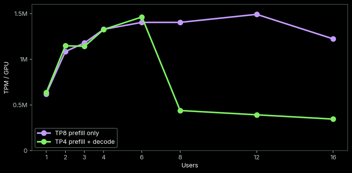
However, choosing TP4 left us extremely constrained on KV cache capacity.
So from here, we turned to strategies to alleviate this constraint.
We lifted the concurrency bottleneck on throughput with better KV caching.
At ~100k max input tokens per request and running TP4, only around 4 users’ conversations could be scheduled onto a single replica without tanking interactivity. Past that, cache hit rate (CHR) plummeted and interactivity/throughput collapsed as long inputs were recomputed. Recomputation is far, far slower than loading their KV entries from HBM. So we went about creating more space for KV.
Go Marie Kondo on the HBM.
The most direct optimization was to find wasted HBM and give it back to the KV cache.
We took a look at the implementation of the DFlash draft model architecture in SGLang and noticed that it incurred twice the necessary HBM usage.
Specifically, the target model intermediates used as input to the draft model were first collected as a list of pointers and then copied into contiguous memory at the end of the forward pass. We rewrote it to instead pre-allocate that contiguous memory as a buffer and push intermediates to it during the forward pass, cutting the peak load on HBM in half. And we did it without changing the append-based logic, thanks to a bit of Python magic. We upstreamed our changes to SGLang in this PR.
Free up HBM with quantization.
The second easiest way to free up space is to use lower-precision floating point numbers everywhere.
But unlike speculative decoding or reducing waste, lowering precision is not a free lunch. Model outputs can change dramatically, and usually not in a way that is good for application outcomes. You can get an intuition for the impact of block quantization techniques with the visualizer in our LLM Engineer’s Almanac (sample below; block-quantized on the left, original on the right).
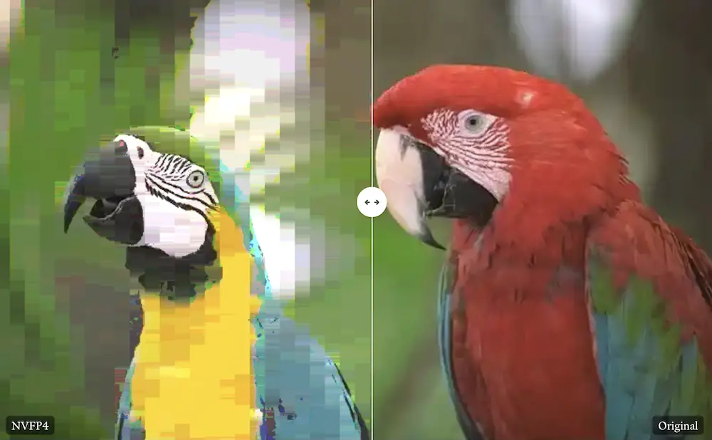
Being able to confidently make changes that are in principle lossy but which don’t impact outcomes for the target application is critical — and a differentiating capability for custom, self-hosted inference applications versus generic, multi-tenant model API providers.
As usual, speculative decoding is the easier case, and so quantizing the draft model is an easy win. The target outcome for the model, decode speed, degrades smoothly, unlike intelligence, and drafter correctness doesn’t impact application outcomes outside of performance. We upstreamed FP8 support for the DFlash speculator architecture to SGLang in this PR.
But there are inevitably appealing optimizations that do impact application outcomes, which is why we’re investing heavily in building our capacity to evaluate the modeling capabilities of inference servers (more on that soon!). We also massively appreciate and support initiatives like Moonshot’s Kimi Vendor Verifier that help consumers of models consistently assess quality. Evals, evals, evals!
Based on our evals, we found that we could quantize the model’s KV cache from BF16 to FP8. This doubles the cache capacity, counted in tokens. Furthermore, most of the expert matmuls were already in NVFP4, the most compact format with native hardware support (for now!). But not the critical “shared” experts that are activated on every token. We found that we could quantize the shared experts from FP8 to NVFP4, freeing up additional HBM for cache. Neither of these changes meaningfully degraded model quality (relative to run-to-run non-determinism) in our evaluations.
Expand KV cache capacity with HiCache
Finally, what if the cache was bigger, even if that meant it was slower?
So far, we’ve only considered GPU HBM for storing KV. That means our two options when handling input sequences are either “keep it in ultra-fast, ultra-expensive storage on the GPU” or “chuck it in the bin”. This leads to a very sharp degradation in replica performance when the KV cache size we need to service the workload exceeds what fits in HBM due to a reduction in cache hit rate (CHR):
That’s why all good caches are multilayer! Each layer of the cache adds another, gentler step down in CHR with load. SGLang’s HiCache expands KV cache capacity by adding “L2” and “L3” cache tiers, allowing KV to be stored in host memory (L2) and distributed storage (L3).
Higher cache tiers are still slower (or else we’d just use them as the lower tier!), so they can easily harm latency and potentially hurt throughput. We got a lot from using just the CPU RAM-based L2 cache. Even then, we essentially only use it to handle excess load.
That is, without HiCache, rapid degradation in performance with concurrency above the level that supported peak performance prevented us from trying to serve at that peak. With it, replica behavior was smoother when an individual replica’s load transiently exceeded the peak.
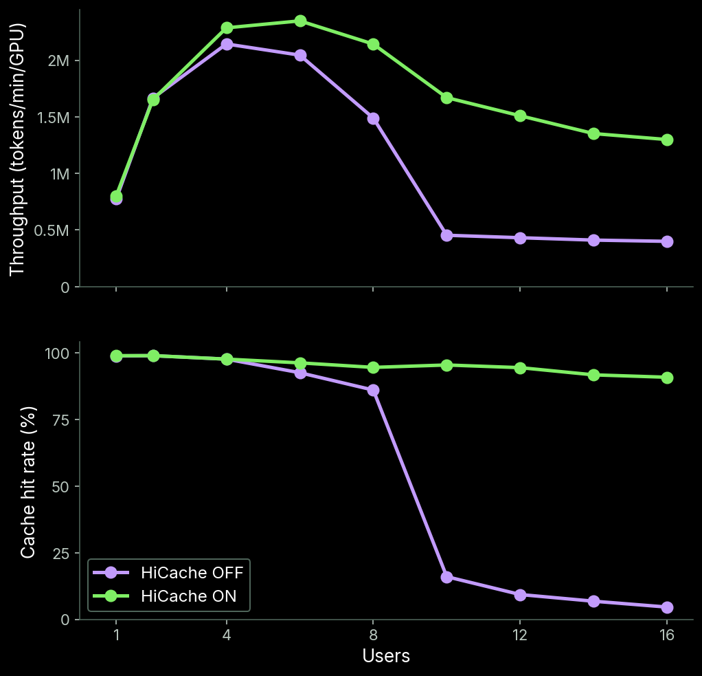
Replicas don’t always have exactly the target request load because of nondeterminism in upstream user/agent behavior and because of routing of requests across replicas, which we consider next.
Finally, scale to many replicas.
After optimizing single-replica performance, we scaled up to a larger deployment — after all this effort, we want to serve significantly more than six concurrent users! At a high level, we do this by serving an autoscaling pool of inference engine replicas behind a Modal Server.
Because our core platform’s autoscaling infrastructure handles all of the typical problems that bedevil autoscaling and entangle it in spaghetti Kubernetes YAML — deciding when to scale, acquiring resources, spinning up a host environment, setting up replicas quickly, recovering from faults, providing observability, releasing resources — essentially the entirety of our work was in the routing layer.
Routing is “easy” except when replicas have state, and the KV cache adds state to the replicas. Luckily, it’s the good kind of state, an ephemeral cache: it’s not necessary for application correctness and can be readily recomputed on a miss. But recomputing incurs a performance penalty, so routing becomes an important part of performance optimization.
We observed two performance problems that caused us to look closer at our routing:
- There were recurring spikes in queued requests and tail time-to-first-token (TTFT) and end-to-end (e2e) latencies.
- Per-replica throughput was lower than expected.
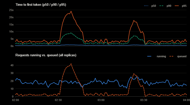
The underlying cause of both of these issues was “regrettably cold prefills” — input sequences that overlapped with sequences we’d seen before, but for which we ended up recomputing the entire KV. The underlying cause of that was inefficient request placement by our original stateless routing algorithm, driven by both concurrency within sessions and unlucky hashing.
Based on this work, we’ve updated our routing layer to support stateful and KV cache-aware routing algorithms. If you're interested in using it with your Modal Servers, reach out.
We started with stateless “session-affinity” routing.
By default, Modal Servers use uniform random routing for all requests. To make certain requests “stick” to a particular container, clients can provide a header, Modal-Session-Id. This is then hashed and mapped onto a replica, something like this:
Though not exactly the circular hashing in the diagram — we use consistent hashing to get better behavior when the replica count or identity changes. See this code sample for details.
Coding agent clients of inference services on Modal can therefore create and re-use session IDs within the same agent session to map requests onto replicas that have already seen their previous inputs and so may have their KV representations in cache, resulting in better performance — usually.
Scale can’t save you from “unlucky” hashing.
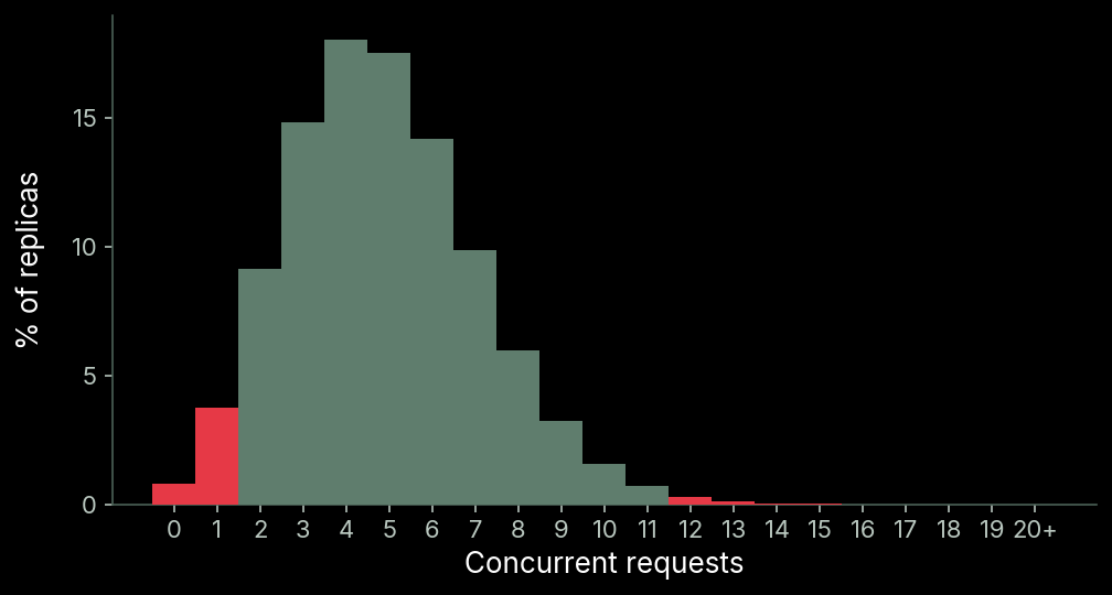
A stateless, uniform-random session routing algorithm works reasonably well for achieving balance when the number of concurrent users is large and when tolerance for variability in concurrent session count is high, but it has some issues with tight tolerance on low concurrencies — the exact regime that high interactivity coding agent inference operates in.
Here’s the math, in sketch. The distribution of session counts for each server using any uniform random hashing algorithm is binomial, with N equal to total session count and p equal to one over server count. The binomial distribution converges quickly to a Poisson distribution with rate parameter equal to Np, aka number of sessions divided by number of servers. Focusing on steady state dynamics, we can treat this as fixed and equal to the target concurrency, thanks to autoscaling. That’s good! But the Poisson distribution has variance equal to this fixed rate parameter, which means the spread in session count per replica does not decrease with increasing scale. It stays fixed, and that gives you predictable tail behavior.
Concretely: if you are targeting five sessions per replica and you have fifty replicas serving 250 sessions, a uniform random routing algorithm will produce a replica serving ≤1 sessions with probability ~4%, which shows up as reduced aggregate efficiency. It will furthermore produce a replica serving at least 12 sessions with probability ~0.5%, which shows up as tail latencies. These rates are independent of scale.
So these routing algorithms can only work in cases where this level of dispersion in load is tolerable — which is not the case for coding agent workloads.
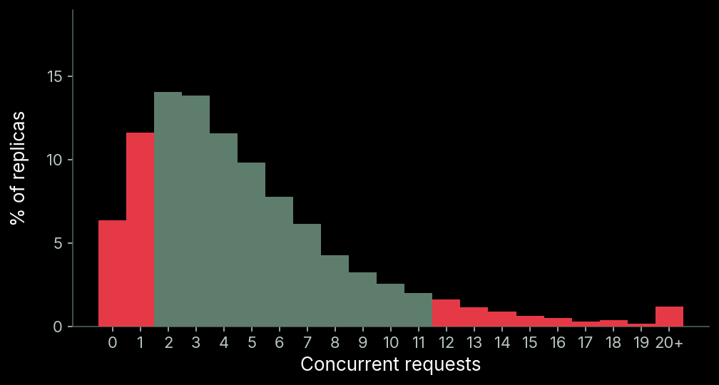
And the situation in practice is in fact worse than the modeling predicts. Deviations from the model (and there are always deviations!) cause extra variance in concurrency counts. We observed this directly. Variance was often several times the mean, with a very heavy right tail that led to occasional very high latencies. See the load-per-replica observations below (from a deployment with its target set to five concurrent requests, for increased interactivity).
This was the root cause of our observed tail TTFT latencies and throughput shortfall.
We rewrote our routing system to handle coding agent workloads better.
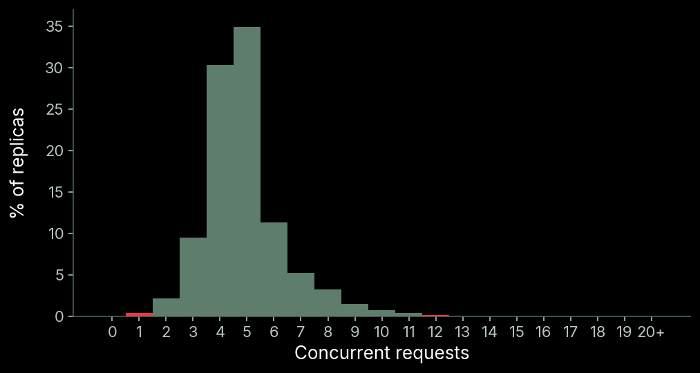
The final router system achieved strongly sub-Poisson dispersion of load (variance under half the mean). A sample load distribution is shown below, again for a deployment targeting five concurrent requests.
To get there, we investigated the causes of tail latencies and over-dispersion of load and added new routing algorithms to address each of them.
- Sessions sending multiple concurrent requests overloaded their replicas. This was fixed by splitting these “thicc sessions” across multiple replicas.
- The work per session was not uniform. This was fixed by making the routing load aware — which also reduces the “unlucky hashing” described above.
- During scale-ups, we rebalanced too many sessions. This was fixed by mapping new sessions preferentially onto new replicas.
Fix hot replicas by breaking up concurrent sessions.
The single biggest cause of over-dispersion and tail latencies was violation of our model of ID’d sessions as “closed-loop”, aka one request at a time per session.
In our system, clients control session IDs, so there’s no way to prevent clients from submitting multiple concurrent requests with the same session ID. And if session IDs are always mapped onto the same container, then the number of concurrent requests per container is no longer bounded. One replica gets “hot”, with very high load, even though overall load is not increased.
Typical coding agent sessions, even with sub-agents, don’t need to share the session ID across concurrent requests, because the typical session proceeds one turn at a time. But there are cases where multiple concurrent input sequences share a prefix. This happens when coding agent sessions are tree-structured, rather than chain-structured — like when you use /btw.
Here’s a point-in-time sample of request count by session ID across a number of replicas, with the session with the largest request count in red. The largest session on replica 6 has a number of concurrent requests several times in excess of the target load. Not good!
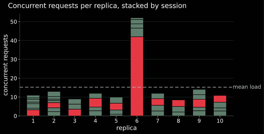
When there are such “thicc sessions”, trying to preserve perfect locality results in worse perf than duplicating some cache and spreading concurrent work across replicas. To fix this, our router intentionally breaks up highly concurrent sessions into multiple containers. That is, before sending a session to one of its assigned replicas, we check a load threshold for that session. We send this request to a different replica when the threshold is exceeded.
Fix unlucky routing and uneven sessions by using fine-grained load-aware session placement.
As described above, uniform-random algorithms are subject to a fixed rate of “unlucky” containers/users.
Even worse, though, the model above assumes that request processing time is fixed as a function of load. But more work means it takes more time to process the work in-flight, and so requests on loaded servers take longer, their load is elevated for longer — thicker tails than in the modeling.
And on top of that, it assumes sessions require equal amounts of work. But some coding agent sessions are long, and the requests in those sessions have many hundreds of thousands of tokens, while others are short and only have a few thousand tokens.
To avoid this, we assign new sessions to replicas according to finer-grained load-based signals, such as running requests (not just assigned sessions!) and KV utilization. We still maintain session affinity after session placement to preserve CHR.
Minimize cache relocation on scale-ups.
During increases in load, we need to increase the number of replicas. The existing replicas have warm cache for the sessions already in-flight, so we’d prefer to keep routing those sessions there.
But with rendezvous hashing, changing the set of containers causes a re-balancing of in-flight sessions, not just new sessions. It’s not a total free-for-all — the point of using consistent hashing-style algorithms is to reroute only the ~1/N of the sessions you need to achieve balance when you add a new target. But even this requires lots of KV recomputation and slowdowns for certain sessions.
This ends up becoming another form of load-aware routing. Especially during load increases, new sessions are generally being created regularly, and mapping more of these onto replicas with less load leads to them preferentially landing on newer replicas: those replicas haven’t accumulated any load yet! There often still needs to be some balancing when the rate of new sessions and new replicas doesn’t match. We again solve this by load-awareness, this time in session reassignment, not just session/request assignment.
Deploy and enjoy.
With all these changes to the routing in place, the behavior of our multi-replica deployment was much closer to what we expected from extrapolating single-replica results. TTFT was substantially more stable, and per-replica throughput stayed much closer to the single-replica performance, even as the deployment grew.
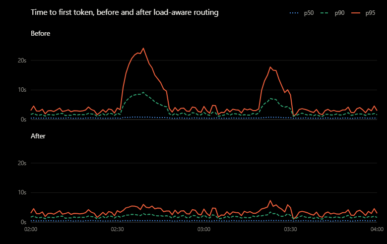
Taken together, these optimizations allowed us to operate multiple Kimi K2.6 inference services at the scale of hundreds of billions of tokens per day and at an interactivity and cost-performance substantively in excess of both our baseline and other offerings.
We have since repeated this basic motion — much faster, because we are much wiser and because we built reusable tools and infra! — for a number of additional models. That includes Moonshot’s updated Kimi K3 model. We repeatedly served the plurality of Kimi-K3 tokens on the competitive OpenRouter marketplace, which routes demand to providers based on the quality of their supplied inference service.
“Science is a liar sometimes.”
Throughout this work, we spent almost as much time on understanding our benchmarks and workload as we did on optimizing the service itself. Benchmarking is hard!
Nearly every metric we cared about was a function of both the system and the workload we fed it. Changing the data could change the results we observed without any changes to the system.
The simple answer to that is to always benchmark on the same data, and for that data to exactly match the workload from production. But production data is sensitive, which limits access. And production data has variability, both across requests and across time, and to do proper performance engineering, it is critical to understand how the system behaves in specific scenarios, not just in aggregate.
So we also want to sometimes run “controlled experiments” outside of the behavioral regime exercised regularly by production to 1) theory-build and 2) clearly isolate and measure the impact of performance interventions. As one example, already mentioned, we ran TP8 in prefill-only mode to clearly demonstrate it was inferior to TP4 in our setting. Consider this analogous to how scientists study systems not merely by observation of natural behavior, but also by intervention in controlled laboratory settings.
A few cases where data-dependence showed up:
- TPM / GPU depends on output length — in a closed loop setting, many “typical” requests may complete in the time required to generate one long sequence.
- Speculative accept length depends on the data it’s evaluated on — code can have roughly 2x the accept lengths of prose.
- CHR depends on individual trajectories — cache-unfriendly patterns like post-hoc edited messages can make caching improvements appear ineffective.
Then what?
This work began with optimizing coding agent workloads for a specific model for one customer. But we’ve also worked on a variety of inference workloads, like high-latency/throughput-sensitive analytical processing (more on that soon). We continue to partner closely with some of the world’s leading companies deploying inference to production, and we’d love to work with you too! Contact us here.
As indicated by the genericity of the performance discussion in this post, this work readily translated to supporting other customers and to serving other models too. It has also motivated longer-term improvements to our inference serving and evaluation stack, including our own eval platform, new routing systems, and better benchmarking techniques, which we’ll talk more about soon.
You may have noticed that we’re quite fond of our core autoscaling cloud infrastructure platform, and we credit it with making possible many of the lower-level engineering choices in this post.
That’s why the post exists at all — if we truly believe our platform is the best for running high-performance inference, why hide inference perf “alpha”? And that’s why we’re committed to open source. Not only did we upstream our work on the inference engine, we also released the code and configuration as the backing source for Modal Auto Endpoints. Spin up a Dedicated Endpoint for Kimi K2.6 right now with modal endpoint create and you’ll be able to inspect our setup — or modify it for your own purposes.
Finally, if you made it this far, we bet you’re interested in and capable of pushing the frontier of inference performance. Check out modal.jobs if you’d like to do that with us! We’d love to hear from both systems engineers with an interest in inference and from inference specialists.
Acknowledgements
This work would not have been possible without the amazing work of open weights model providers like Moonshot AI, open source inference engines like SGLang, and the entire community of researchers and engineers who share their work for others to build on.