Multi-token Residual Prediction
Editor's Note: this guest blog post describes the results of a research collaboration between Modal Research and NYU Shanghai's HeavyBall Research.
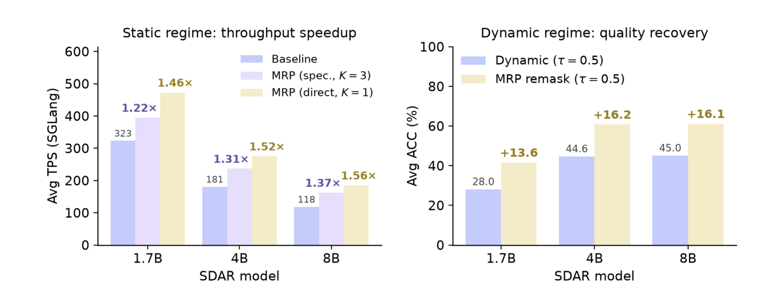
MRP is one small module with two uses. Left: in the static regime, it accelerates decoding losslessly (speculative, lookahead steps K = 3) or further still with a small quality cost (direct, lookahead steps K = 1), reaching up to 1.56× throughput in SGLang. Right: in the dynamic regime, it recovers up to +16 accuracy points lost to aggressive low-threshold decoding (threshold τ = 0.5). Averaged over GSM8K, MATH500, HumanEval, and MBPP on SDAR-1.7B/4B/8B.
TL;DR: Multi-Token Prediction (MTP) speeds up autoregressive models by predicting several tokens from a single forward pass (Gloeckle et al., 2024). We bring this idea to diffusion language models, with one change that makes it work: instead of training a small head to predict the next denoising step's full distribution, we train it to predict the residual between adjacent steps. The residual is a much easier target, so a tiny module can predict it accurately and apply it across several steps. The same module then serves both of the regimes that DLM inference normally has to trade off against each other: in the static regime it gives (near-)lossless speedup when output quality must be preserved (averaging up to 1.56× in SGLang), and in the dynamic regime it recovers most of the quality lost to aggressive throughput settings (up to +16 points on average).
Paper: https://arxiv.org/abs/2605.18817
Code: https://github.com/heavyball-research/multi-token-residual-prediction
SGLang implementation: https://github.com/heavyball-research/sglang
Models: https://huggingface.co/collections/heavyball/sdar-mrp
Starting from MTP
If you’ve been anywhere near fast LLM inference, you know the multi-token prediction (MTP) story. Autoregressive models generate one token per forward pass, and that’s expensive. So people bolt on lightweight heads, à la Medusa, EAGLE, DeepSeek’s MTP, that peek at the backbone’s hidden states and guess the next few tokens in one forward pass. Pair that with speculative verification, and we get real speedups.
It’s a beautiful idea, and it works. So naturally we asked: can we make it work beyond autoregressive models?
Diffusion LMs (DLMs) are a natural place to look, because they don't decode left to right. A DLM starts from a fully masked sequence and denoises it, unmasking high-confidence positions a few at a time. Parallelism is built into the process, but with a tradeoff: unmask too many tokens in a single step and quality drops, because each token is decoded without seeing the others committed alongside it. Most of the DLM-acceleration literature lives on this one Pareto curve, trading quality for speed.
This is the tradeoff we wanted to break, and MTP looked like the right tool to do it. If a lightweight head can predict additional tokens from the backbone's hidden states, it could decode several positions per forward pass while keeping each one aware of the others, instead of simply unmasking more and paying for it in quality. The question was whether the MTP recipe would carry over to the diffusion setting. As we found out, it does not transfer directly, and seeing why is what led to our method.
A naïve attempt
We start by taking a small head and distilling it to predict the next step’s full log-density directly from the current step’s hidden states. Run it a few times to unmask several tokens per backbone pass.
The problem shows up the moment we ask the head to take more than one step. Distilling the entire distribution means every step has to reproduce a big, high-dynamic-range target from scratch, and per-step errors compound. We found a head trained this way is fine at one step, but by three or four steps it has collapsed at every model scale we tried. On the SDAR-4B backbone, our direct-distillation head went from 84.8% GSM8K at one step to single digits at four. It just couldn’t hold the distribution together across iterations.
| Method | K=1 | K=2 | K=3 | K=4 |
|---|---|---|---|---|
| Naïve MTP | 84.8 | 16.9 | 5.9 | 1.9 |
GSM8K (0-shot, CoT) accuracy on SDAR-4B. We apply the MTP recipe directly here and the accuracy drops sharply beyond the first MTP step. Here K denotes the prediction steps.
The main insight
The failure above is also a clue. If the full next-step distribution is hard to predict across multiple steps, the question is whether there is an easier target to predict instead. There is, and it comes from looking at how little the backbone's output actually changes between two adjacent denoising steps.
That’s the whole insight, and it changes the target. We don’t need a small module to reproduce the next step’s full distribution from scratch. We need it to predict a small correction to a prediction that’s already pretty good.
And this isn’t just a lucky empirical fact. It falls out of the Markov structure of denoising: each step perturbs only a handful of positions, so by a Lipschitz argument the predictive distribution at the untouched positions can only move so far, and the bound tightens as denoising progresses and the model grows more confident. The signal we’re asking a small module to learn is genuinely low-complexity. Which is exactly why a small module can learn it.
Multi-token Residual Prediction (MRP)
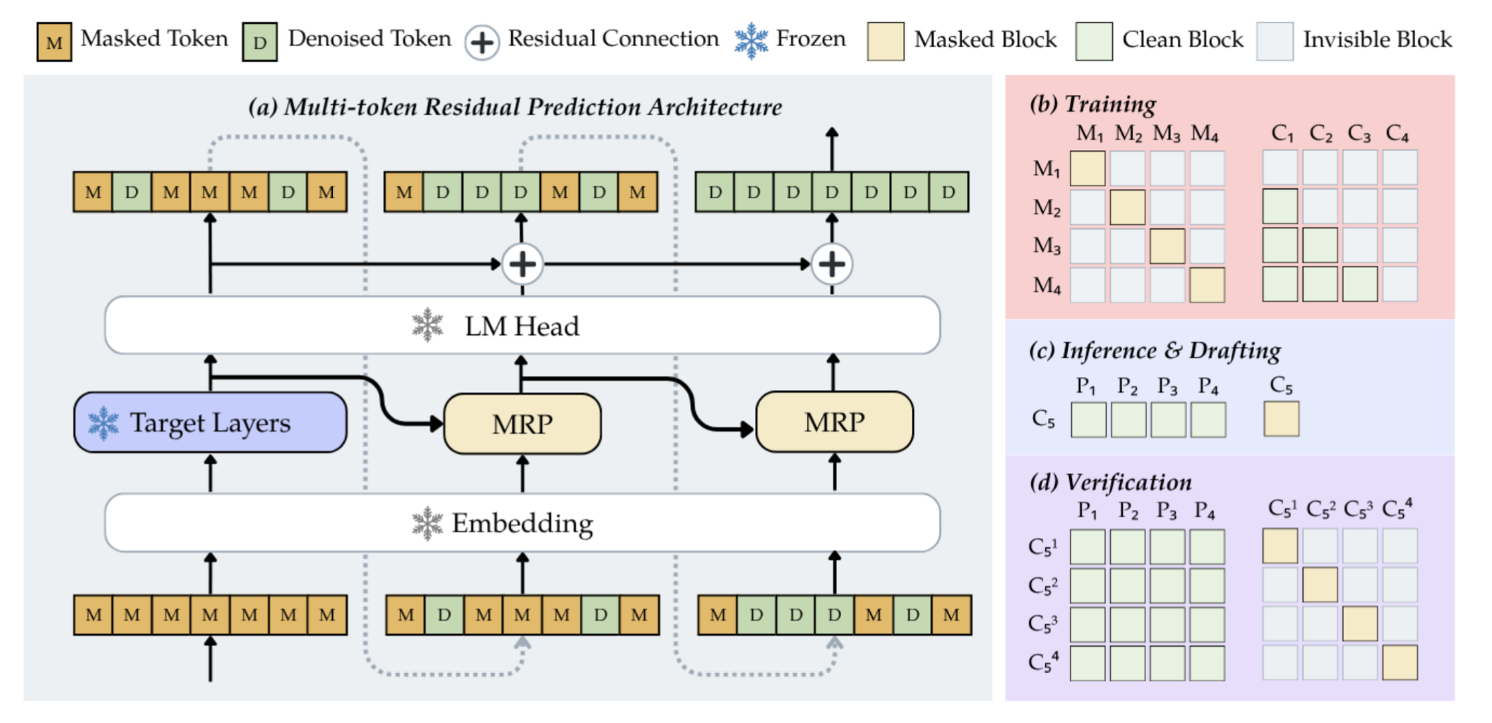
Multi-Token Residual Prediction (MRP) is a small transformer (3 layers in our main configuration) attached to a frozen DLM backbone. It reads the backbone's hidden states, predicts the inter-step logit residual, and adds it to the backbone's own logits. The backbone, its LM head, and its token embeddings stay frozen; only the MRP module is trained.
The training objective is a residual version of the MTP distillation loss. We run the frozen backbone twice, once before and once after revealing a set of tokens, and train MRP with a KL divergence on the still-masked positions to minimize the difference between the two outputs. Because the normalizing constants cancel under the softmax, this is equivalent to matching the true conditional distributions, while the module itself only ever represents the correction.
| Method | K=1 | K=2 | K=3 | K=4 |
|---|---|---|---|---|
| Naïve MTP | 84.8 | 16.9 | 5.9 | 1.9 |
| MRP | 88.6 | 84.9 | 70.9 | 57.2 |
GSM8K (0-shot, CoT) accuracy on SDAR-4B. Using the auxiliary module to predict the residual rather than the entire distribution makes the learning much easier. Here K denotes the prediction steps. The benefit of the residual framing shows up as K grows. The gap between directly modeling the distribution (Naive MTP) and residual learning (MRP) are within a few points of each other at K = 1, but diverge sharply beyond that: at K = 2, residual learning already leads by +65 points on GSM8K, and the direct variant collapses entirely by K = 4.
Applications in inference
With one trained module on a frozen backbone, we can cheaply approximate what the next denoising step would produce. How that approximation is best used depends on how the backbone is being decoded.
DLMs are typically run in one of two regimes. In static denoising, each step unmasks a small, fixed number of positions; this keeps quality high but throughput low, and is the regime you want when the output has to be right. In dynamic denoising, every position whose confidence clears a threshold is unmasked at once; this pushes throughput up, but at low thresholds the backbone commits many tokens per step and quality degrades.
MRP applies to both regimes, but it plays a different role in each: in the static regime it adds reveals to go faster; and in the dynamic regime it revokes over-eager reveals to recover quality.
Application I: Lossless speedup in static denoising
In the static regime, MRP turns inference into a dial you can turn. The same trained module gives you a spectrum of operating points, from exactly the backbone's output to substantially faster with a small, measurable quality cost, and you pick where to sit based on what your application actually needs.
At one end is speculative decoding, for when the output has to match exactly what the backbone would have produced. Here MRP acts as a drafter: it cheaply proposes the next batch of tokens, and the backbone verifies them in a single pass. Positions where the backbone agrees with the draft are accepted; positions where it disagrees are remasked and redone. Because diffusion models score every position in one forward pass, this position-wise verification is natural. The verification pass is not wasted: its hidden states and logits seed the next iteration, so when the acceptance rate is high it doubles as the next step's backbone pass and its cost is amortized.
| Backbone | GSM8K | MATH500 | HumanEvall | MBPP |
|---|---|---|---|---|
| SDAR-4B | 90.0 / 1.36x | 68.0 / 1.26x | 67.7 / 1.35x | 66.5 / 1.27x |
| SDAR-8B | 90.4 / 1.40x | 74.8 / 1.39x | 72.6 / 1.34x | 67.3 / 1.34x |
Speculative mode in SGLang. Accuracy (%) followed by throughput speedup over the backbone-only baseline. Quality matches the backbone by construction. Measured on a single H100; an implementation we provide in SGLang.
At the other end is direct decoding, which skips verification and commits MRP's corrected logits directly. Verification costs a full backbone forward pass, so dropping it raises the ceiling on speedup, and the residual predictions are accurate enough on their own that, on reasoning tasks, the quality cost is small:
| Setting | GSM8K | MATH500 | HumanEval | MBPP |
|---|---|---|---|---|
| Baseline | 90.9 / 1x | 72.2 / 1x | 73.8 / 1x | 67.7 / 1x |
| Direct (MRP Step 1) | 90.1 / 1.59x | 71.4 / 1.61x | 67.1 / 1.53x | 63.8 / 1.51x |
| Direct (MRP Step 2) | 89.2 / 1.89x | 70.8 / 1.91x | 64.0 / 1.78x | 59.9 / 1.75x |
Direct decoding on SDAR-8B. Accuracy (%) followed by throughput speedup over the backbone. Tokens are committed without verification. K sets how many MRP steps run per backbone forward, so it is itself a knob: K = 1 stays within a point of the backbone on reasoning at 1.6×, K = 2 pushes past 1.8× for a larger drop on code tasks. Smaller scales follow the same pattern (full tables in the paper).
The key is that you choose the operating point. Lossless when correctness is non-negotiable, faster when latency dominates and a small quality cost is acceptable, tuned per task and even per request. That control only exists if you own the inference stack for your application. Behind a closed API, this tradeoff is made for you: the provider fixes the decoding policy, and you take whatever cost–quality point they ship. Running your own backbone with MRP puts the dial back in your hands.
Application II: Quality recovery
Now consider the opposite regime: an interactive setting where latency matters most, so the unmasking threshold is set low and many tokens are revealed per step. At aggressive thresholds this hurts, because the backbone commits a batch of tokens in one step, each chosen before it can account for the others being committed alongside it.
Here MRP runs in the other direction. After the backbone over-reveals at the low threshold, a single MRP pass predicts the residual conditioned on those fresh reveals, and the corrected logits re-evaluate the tokens just committed. Any token whose confidence now falls below the threshold is remasked and deferred to a later step with more context. Because the residual encodes how each prediction shifts once its new neighbors are accounted for, MRP identifies the reveals that were only confident in isolation. The same threshold τ gates both the reveal and the remask, so no additional tuning is introduced.
| Model | τ | GSM8K | MATH500 | HumanEval | MBPP |
|---|---|---|---|---|---|
| 1.7B | 0.5 | 41.6 → 59.1 (+17.5) | 26.0 → 37.4 (+11.4) | 17.7 → 28.7 (+11.0) | 26.9 → 41.3 (+14.4) |
| 1.7B | 0.6 | 56.3 → 67.0 (+10.7) | 33.4 → 40.4 (+7.0) | 31.7 → 43.3 (+11.6) | 42.4 → 49.0 (+6.6) |
| 1.7B | 0.7 | 65.4 → 71.8 (+6.4) | 39.4 → 48.6 (+9.2) | 40.9 → 45.1 (+4.2) | 49.8 → 51.0 (+1.2) |
| 1.7B | 0.8 | 70.6 → 75.4 (+4.8) | 47.4 → 52.0 (+4.6) | 45.7 → 48.8 (+3.1) | 51.8 → 51.8 (0.0) |
| 1.7B | 0.9 | 76.2 → 77.3 (+1.1) | 51.2 → 57.0 (+5.8) | 49.4 → 52.4 (+3.0) | 53.7 → 54.1 (+0.4) |
| 4B | 0.5 | 63.4 → 81.1 (+17.7) | 44.2 → 58.4 (+14.2) | 32.3 → 53.1 (+20.8) | 38.5 → 50.6 (+12.1) |
| 4B | 0.6 | 76.4 → 85.5 (+9.1) | 53.6 → 61.4 (+7.8) | 49.4 → 57.9 (+8.5) | 49.8 → 57.2 (+7.4) |
| 4B | 0.7 | 84.6 → 88.5 (+3.9) | 60.4 → 65.6 (+5.2) | 60.4 → 62.2 (+1.8) | 61.1 → 63.4 (+2.3) |
| 4B | 0.8 | 87.9 → 90.1 (+2.2) | 66.8 → 70.6 (+3.8) | 64.6 → 62.8 (−1.8) | 63.8 → 64.2 (+0.4) |
| 4B | 0.9 | 88.5 → 90.1 (+1.6) | 69.0 → 70.6 (+1.6) | 67.1 → 65.9 (−1.2) | 65.4 → 64.6 (−0.8) |
| 8B | 0.5 | 67.9 → 82.3 (+14.4) | 45.2 → 58.0 (+12.8) | 32.3 → 54.9 (+22.6) | 34.6 → 49.4 (+14.8) |
| 8B | 0.6 | 79.6 → 86.8 (+7.2) | 54.8 → 63.8 (+9.0) | 48.8 → 63.4 (+14.6) | 48.3 → 59.9 (+11.6) |
| 8B | 0.7 | 85.9 → 89.0 (+3.1) | 60.8 → 69.0 (+8.2) | 64.6 → 72.6 (+8.0) | 54.9 → 60.3 (+5.4) |
| 8B | 0.8 | 89.3 → 91.0 (+1.7) | 68.0 → 70.2 (+2.2) | 74.4 → 75.0 (+0.6) | 62.3 → 66.5 (+4.2) |
| 8B | 0.9 | 90.8 → 91.4 (+0.6) | 70.0 → 72.0 (+2.0) | 75.0 → 75.0 (0.0) | 66.9 → 68.5 (+1.6) |
MRP remasking improves the accuracy of low-threshold dynamic decoding. For each SDAR backbone (1.7B / 4B / 8B) and unmasking threshold τ, each cell shows plain threshold-based Dynamic decoding → MRP Remask. The same τ gates both the reveal and the remask, so no extra tuning is introduced. Gains are largest at aggressive (low) thresholds, where the backbone over-commits and remasking has the most to revoke (up to +22.6 on 8B HumanEval at τ = 0.5), and shrink toward zero as τ rises and the backbone already unmasks conservatively. Reasoning (GSM8K, MATH500) improves at every operating point; the rare small regressions are confined to code at high τ. Accuracy in %.
The idea of revisiting freshly revealed tokens and remasking the ones that no longer hold up appears in prior work such as DMax, RCD, and WINO. What is new here is the signal MRP uses to make that decision. Rather than spending a second backbone pass to re-evaluate the reveals, MRP reads the inter-step residual, which already encodes how each prediction shifts once the new tokens are accounted for, and remasks the positions whose corrected confidence falls back below the threshold. The re-check that those methods pay a full backbone forward for, MRP gets from a single lightweight residual pass.
What we learned
A few things that stood out along the way:
- Depth has a sweet spot at 2–3 layers. Accuracy improves steadily from 1 to 3 layers, then plateaus while throughput keeps dropping, since the extra layers only add per-step latency; by 8 layers the tradeoff is strictly worse. Other speculative-drafting modules settle deeper. For example, DFlash lands around 5 layers, and the difference seems to come from how target-model information reaches the draft module. Those designs use per-layer KV injection, feeding the backbone's hidden states into every draft layer rather than only at the input, so a deeper module keeps benefiting from added depth.
- The best depth depends on the mode. In direct decoding, where MRP's outputs are used as-is, deeper modules help more. In speculative decoding, verification corrects MRP's mistakes anyway, so a shallower and faster module reaches the same final quality at higher throughput.
- MRP composes cleanly. At its core, MRP is just a cheap, accurate prediction of what the next denoising step would produce. That prediction is a primitive other methods can build on, which is why the same module supports both of the schemes in this post, e.g., speculative decoding and remasking. It adds a capability to the ecosystem rather than competing with it.
If you work with diffusion LMs, MRP is easy to attach and gives you a choice you did not have before: lossless and faster, or faster still with the quality you would otherwise lose handed back.
Why we chose Modal
One thing that impressed us the most during the project was the quality of Modal’s infrastructure. It let us test our ideas as modular experiments and focus on the idea rather than infrastructure, which is how we went from hypothesis to an SGLang implementation so fast.
We also built a lightweight tool, modal-ssh, to share Modal workflows across our group. The tool captures a research environment (packages, volumes, secrets, and Git repos) in a small YAML config, then uses it to launch either an interactive VM or a long-running background job. This significantly accelerates the iteration of our projects, as it enables us to share configs across our team, and helps new members get started with Modal with minimal learning cost. The source is available here.
We see this project as the first step in our joint exploration of fast inference, with more kernel and serving-level directions we’d love to push on together.